时域有限差分求解器(FDTD)
SimWorks FDTD 是研究人员和工程技术人员处理各种微纳光电子问题的有力工具。下面,我们会简要介绍求解器的物理原理、求解器的主要特色和求解器的仿真流程。
FDTD算法基本原理
时域有限差分FDTD是从时域麦克斯韦旋度方程出发,在一定体积内和一段时间上对连续电磁场的数据抽样,它直观地再现了在离散数值时空中电磁现象的物理过程。因此,FDTD是对电磁问题的最本质、最完备的数值模拟,具有广泛的适用性。FDTD求解的是麦克斯韦方程组的时域解,借助傅里叶变换,通过一次仿真即可得到器件在宽频中的频域响应。FDTD的基本原理如下:
对于非磁性材料,麦克斯韦旋度方程可以化为:
根据上述方程, 在Yee cell网格上进行FDTD差分离散:
- 使用中心差分近似麦克斯韦微分方程
-
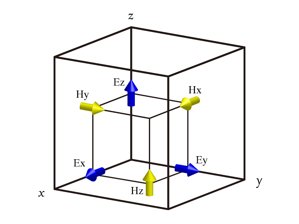
FDTD 中的电磁场基于
Yee cell网格在空间中交错分布 (见下图左)。电场分布在网格棱线中心,磁场分布在网格面中心。每一个电场分量和与它相邻的并且垂直于该电场分量的4个磁场分量,满足麦克斯韦旋度方程(磁场同理)。
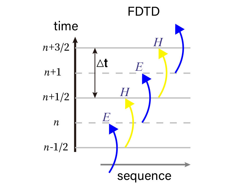
-
FDTD 中离散化的电磁场在时间上是交错迭代,采用蛙跳法逐步递推求解(见下图中)。
-
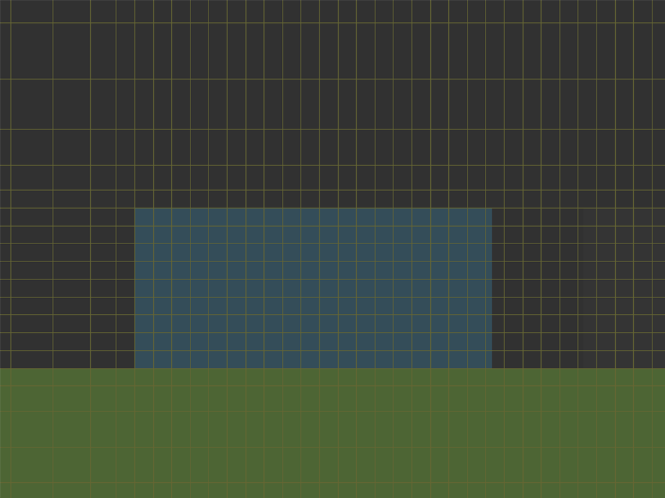
FDTD中 的材料是基于
Yee cell网格进行离散 (见右下图)。越细的网格能够更好的再现结构,但是会导致内存和仿真时间大大增加。由于网格的选取会严重影响器件的仿真速度和精度,我们为用户提供了自动非均匀网格和各种共性网格等高级选项,具体请见mesh。
- 根据空间网格设置,生成平行于直角坐标系的
FDTD网格(通常称为mesh)。 FDTD网格中的材料检测点和结构形状进行点形逻辑判断,得到符合FDTD网格分布的材料(结构对应的电磁材料)离散分布。
- 根据空间网格设置,生成平行于直角坐标系的
因此,数值化后的电磁场三维递推方程如下:
三维的其它方向与上面公式类似,详见参考[1,2]。
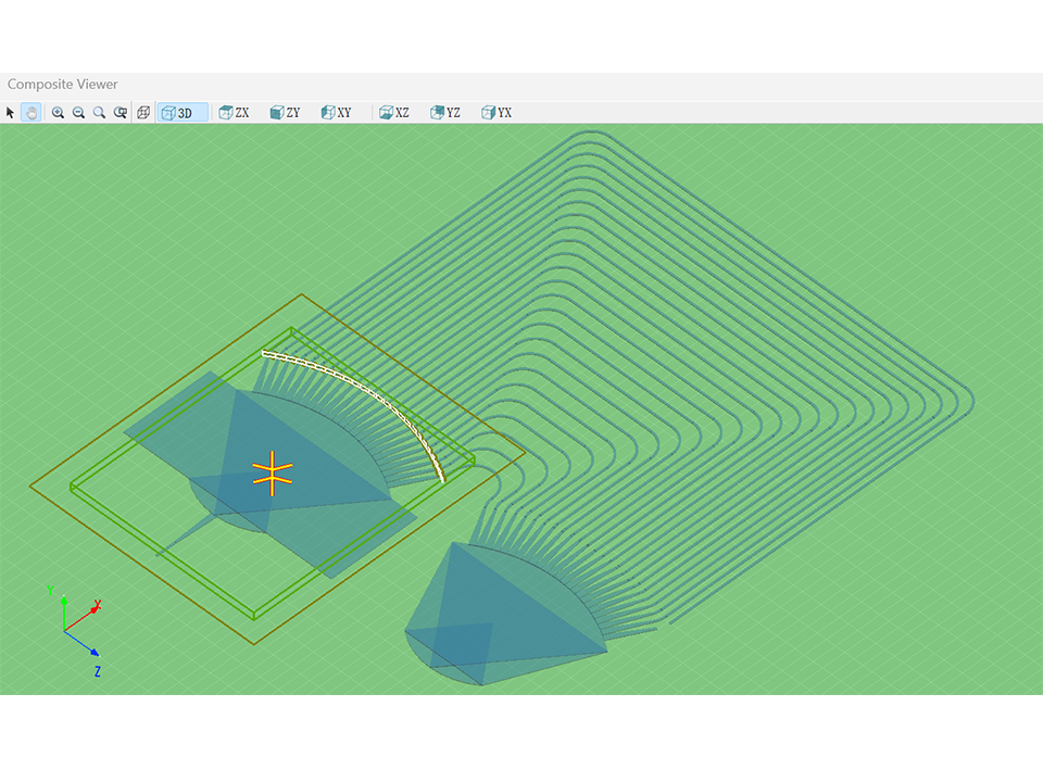
本软件能够实时显示电磁场的时域场图。FDTD仿真后,各个网格点的材料数据、电场/磁场、功率、透过率/反射率等信息也可以直接得到(请见下图)。
_20240919113530A039.png)
求解器的主要特色
3D CAD界面和丰富的零件库
- 多视角3D Computer-aided Design(CAD)工作平台,助力模型搭建。
- 内置丰富的结构库,包括多边形及曲面结构,能够轻松搭建各种复杂结构的器件。
- 支持Graphic Design System(GDS)版图文件的直接导入,方便调整复杂结构。
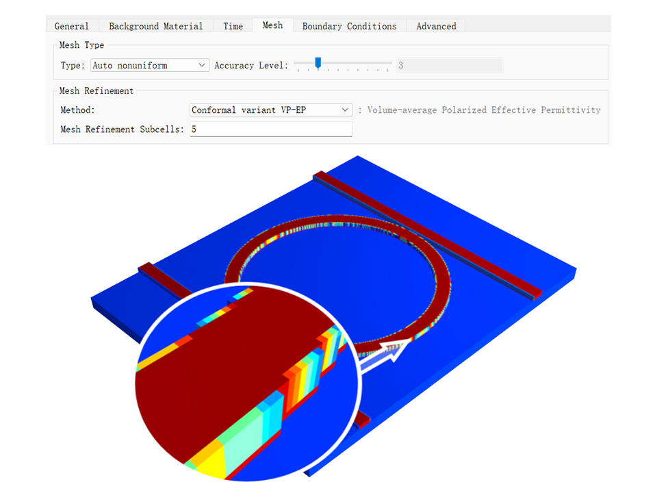
网格技术
- 支持自动非均匀网格、自定义网格等网格剖分技术,提供更高效的仿真。
- 拥有当前流行的高精度共形网格细化技术,包括:体平均偏振相关的等效介电常数法(Volume-average polarized effective permittivity)、体平均法(Volume average)、Yu-Mittra 1、Yu-Mittra 2,以达到更精确的仿真结果。
边界条件
- 提供多种仿真边界条件,如完美匹配层(PML)、周期、布洛赫(Bloch)、对称/反对称、完美电导体(PEC)/完美磁导体(PMC)。
_20240115173008A019.png)
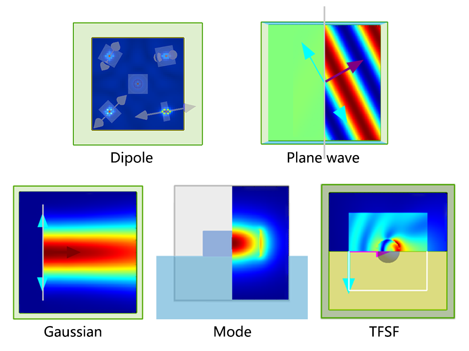
多种光源
- 提供偶极子源、平面、高斯光源、模式源、总场散射场源(TFSF)、导入源等多种注入源类型可供用户选择。
- 轻松满足窄带/宽带、不同入射角度、复杂偏振类型等不同光源的仿真需求。
- Port 端口方便用户在指定模式下提取系统的S参数,S参数随输入/输出模式的不同而变化。
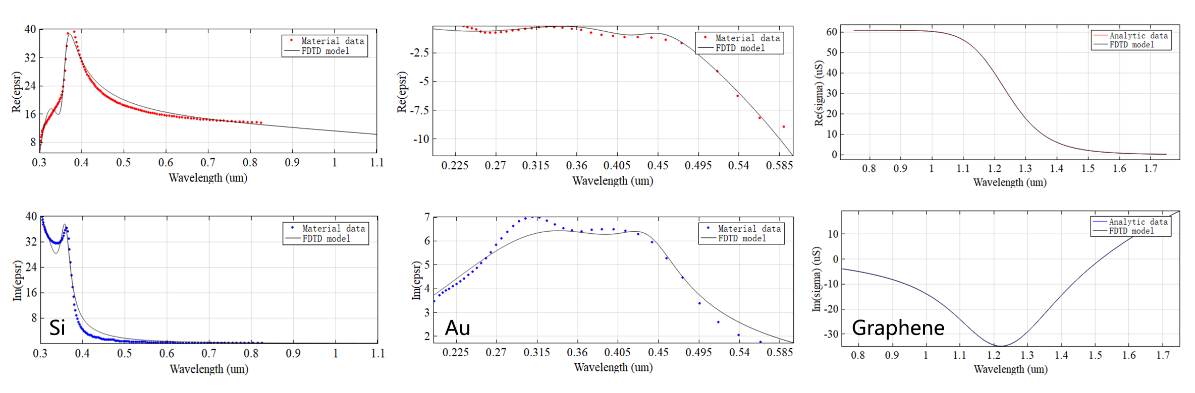
材料属性
- 色散材料的多系数模型精确度高,能够兼容多种材料类型,如Drude模型、Debye模型、Lorentz模型、nk材料等。
- 允许用户导入自定义的散点材料数据,该数据被自动拟合成内置的模型。
- 支持2D材料,例如:石墨烯材料、RLC集总元件、表面电导材料。
- 支持对角各向异性材料及非线性材料的仿真,包括二阶非线性、拉曼效应和克尔效应。
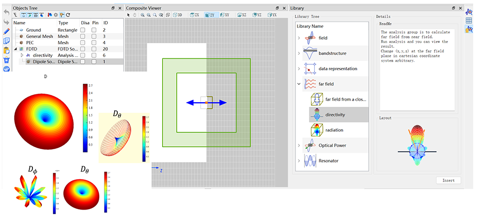
后处理分析
- 功能丰富的后处理分析程序库,包括远场分析、能带结构分析、Q质量因子分析等。
- 模块化的分析组拥有方便快捷的程序编辑窗口,允许用户灵活地自定义各种分析组。
扫描优化
- 支持扫描、优化、S矩阵扫描和嵌套扫描。内置优化算法可自动帮助用户优化器件的设计。
_20240115173926A023.png)
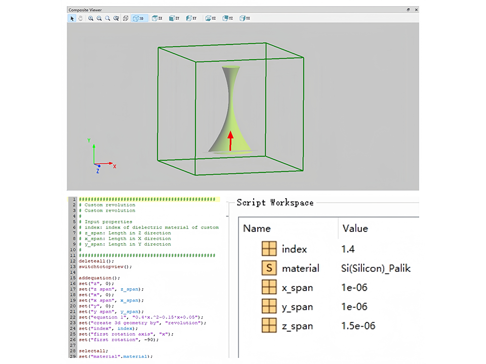
脚本控制
- 脚本功能允许用户操纵仿真中的每一个步骤,实现参数化的构建,为用户提供新的交互体验。
- 软件内置完整的函数库,允许自定义函数,基本满足数学计算的所有需求。
强大的算力
- 在OpenMP、CUDA、MPI、AVX等多种并行计算技术的加持下,算力及运算速度都得到了高效提升。
- 为用户提供云端计算服务,随时随地查看仿真进程,不再局限于本地计算资源。

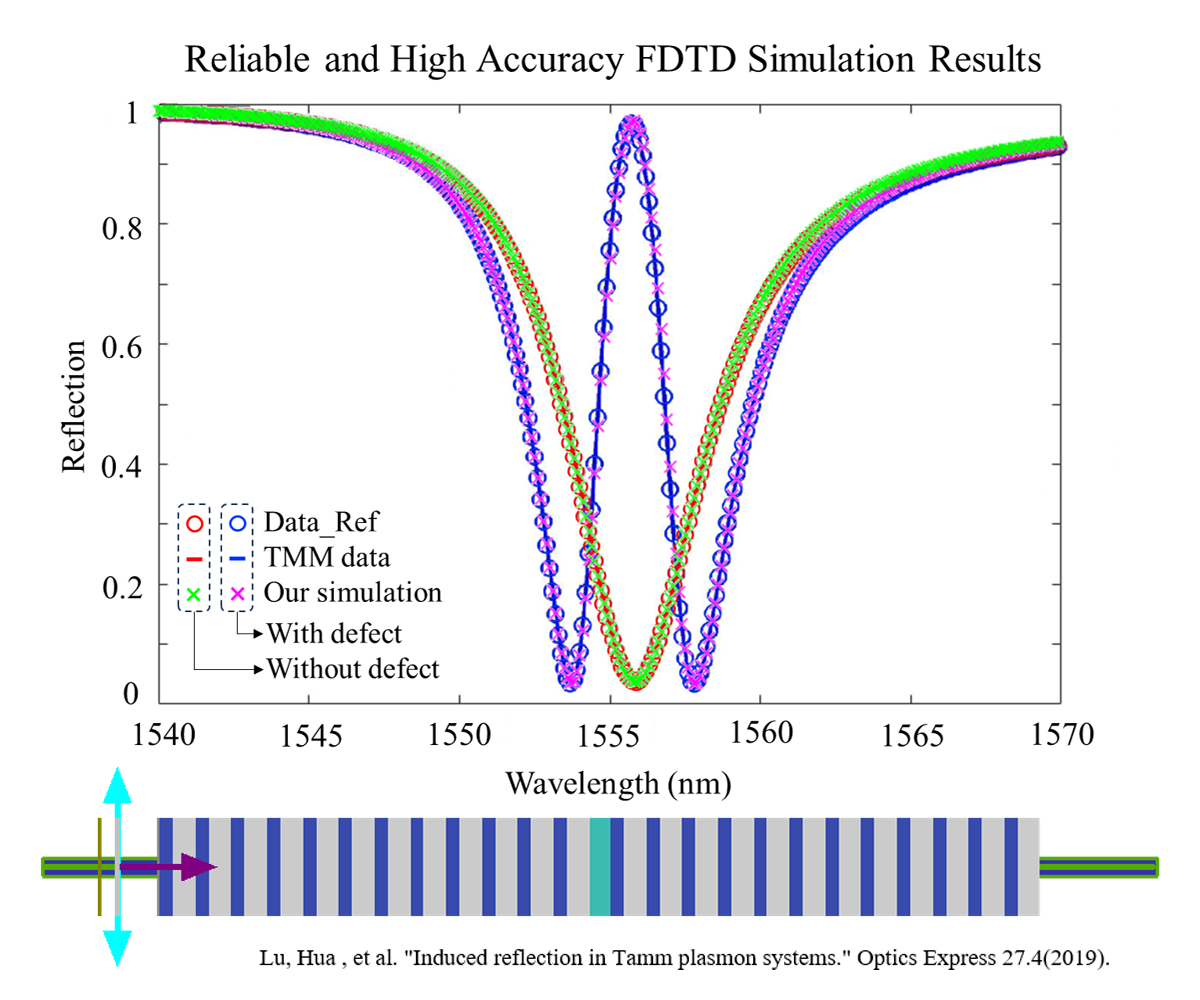
领先行业的超高计算精度
- 软件在不同的结构参数工程中均能获得超高精度的计算结果。以布拉格光栅为例,如下图所示,无论其结构是否存在缺陷,仿真结果均与文献中的数据保持高度一致。
求解器的主要仿真流程
当用户选定要使用的求解器后,仿真任意一个工程简单直接,方便新手快速入门。仿真的主要流程包括如下图展示的步骤。仿真完成后,结果数据可以直接画图展示或者导出到其它关联软件做进一步的分析。
flowchart TB

StructureLibrary( 结构库 )
Material( 材料库 )

SettingTimeSpatial( 设置时空参数 )
SettingMesh( 设置网格 )
SettingBoundary( 设置边界 )
Source(配置光源)
Monitor(配置监视器)
Run(运行仿真)
End[/仿真结束\]
DataVisualizer[(结果可视化)]
isSweep{参数扫描优化?}
Sweep[[扫描优化]]
isPostProcess{后处理分析?}
PostProcess[[后处理分析]]


subgraph obj_sub [配置对象]
  direction TB
  StructureLibrary
  Material
end
subgraph sim_sub [配置求解器]
  direction TB
  SettingTimeSpatial
  SettingMesh
  SettingBoundary
end

subgraph sm_sub [光源和监视器]
  direction TB
  Source
  Monitor
end

subgraph FDTDSolver[时域有限差分求解器]
  direction TB
  Run
  End
end
subgraph post_sub[后处理]
  isSweep --是--> Sweep
  isPostProcess --是--> PostProcess
end
sim_sub --> obj_sub
obj_sub --> sm_sub
sm_sub --> FDTDSolver
Run --> End
FDTDSolver --> DataVisualizer
FDTDSolver --> isSweep
FDTDSolver --> isPostProcess

PostProcess --> DataVisualizer
Sweep -->DataVisualizer
参考文献
[1] Allen Taflove, "Computational Electromagnetics: The Finite-Difference Time-Domain Method", Boston:Artech House, (2005).
[2] John B. Schneider, "Understanding the Finite-Difference Time-Domain Method", www.eecs.wsu.edu/~schneidj/ufdtd, (2010).