频域有限差分求解器(FDFD)
SimWorks FDFD 是研究人员和工程技术人员分析谐振腔的频谱、金属天线等问题的有力工具。下面,我们会简要介绍FDFD求解器的基本原理和主要特色。
FDFD算法基本原理
频域有限差分(FDFD)求解器通过求解频域麦克斯韦方程组来计算在目标频率下的电磁场空间分布。FDFD的基本原理如下。
-
频域麦克斯韦方程组
对于无源材料,麦克斯韦旋度方程具有以下形式:
-
FDFD网格
-
FDFD 中的电磁场基于
Yee cell网格在空间中交错分布,电场分布在FDFD网格棱线中心,磁场分布在FDFD网格面中心。 -
FDFD中的材料是基于
Yee cell网格进行离散,FDFD网格中的材料检测点和结构形状进行点形逻辑判断,得到符合FDFD网格分布的材料(结构对应的电磁材料)离散分布。
-
-
有限差分算法
根据频域麦克斯韦方程,在
Yee cell网格上进行差分离散,对于Y轴向磁场分量有:在空间内沿坐标轴线性展开,可将以上方程转换为如下形式:
同理可知:
其中,、、 和 、、 是包含整个网格中所有电场和磁场分量的列向量;、 和 、 是计算电磁场分量在网格上的空间差分所使用的带状矩阵;和为包含整个网格沿其中心对角线的相对磁导率和介电常数张量分量的对角矩阵。
根据上述方程,将恒定频率下的麦克斯韦方程组转换为矩阵形式:。
矩阵为物理空间中的波动矩阵,列向量为需要求解的电磁场分量,列向量为源。
_20240116095016A033.png)
求解器的主要特色
3D CAD界面和丰富的零件库
- 多视角3D Computer-aided Design(CAD)工作平台,助力模型搭建。
- 内置丰富的结构库,包括多边形及曲面结构,能够轻松搭建各种复杂结构的器件。
- 支持Graphic Design System(GDS)版图文件的直接导入,方便调整复杂结构。

网格技术
- 支持自动非均匀网格、自定义网格等网格剖分技术,提高复杂结构Yee cell网格构建效率。
- 拥有当前流行的高精度共形网格细化技术,包括:体平均偏振相关的等效介电常数法(Volume-average polarized effective permittivity)、体平均法(Volume average)、Yu-Mittra 1、Yu-Mittra 2,以达到更精确的仿真结果。
边界条件
- 提供多种仿真边界条件,如完美匹配层(PML)、周期、布洛赫(Bloch)、对称/反对称、完美电导体(PEC)/完美磁导体(PMC)。
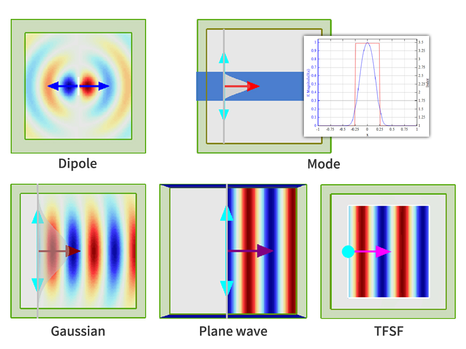
多种光源
- 提供偶极子源、平面源、高斯光源、模式源、总场散射场源(TFSF)、导入源等多种注入源类型。
- 轻松满足不同入射角度、不同偏振类型的光源需求。
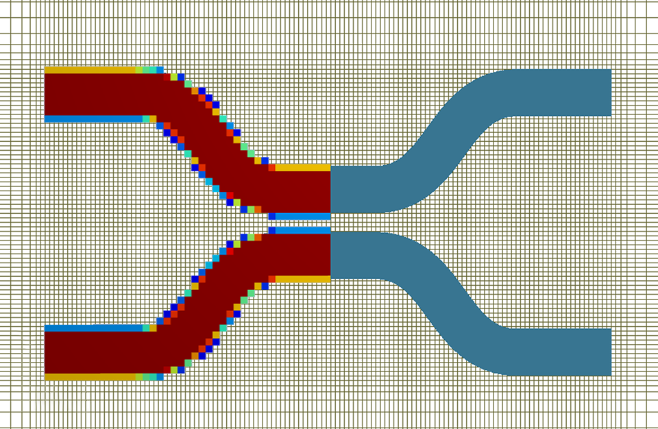
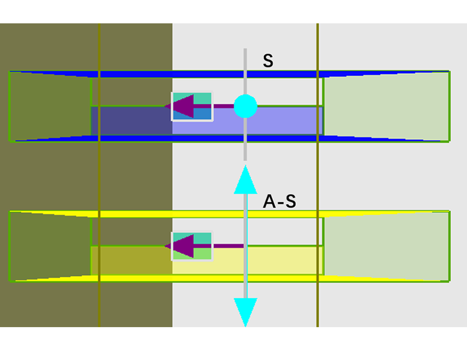
- Port端口方便用户在指定模式下提取系统的S参数,S参数随输入/输出模式的不同而变化。
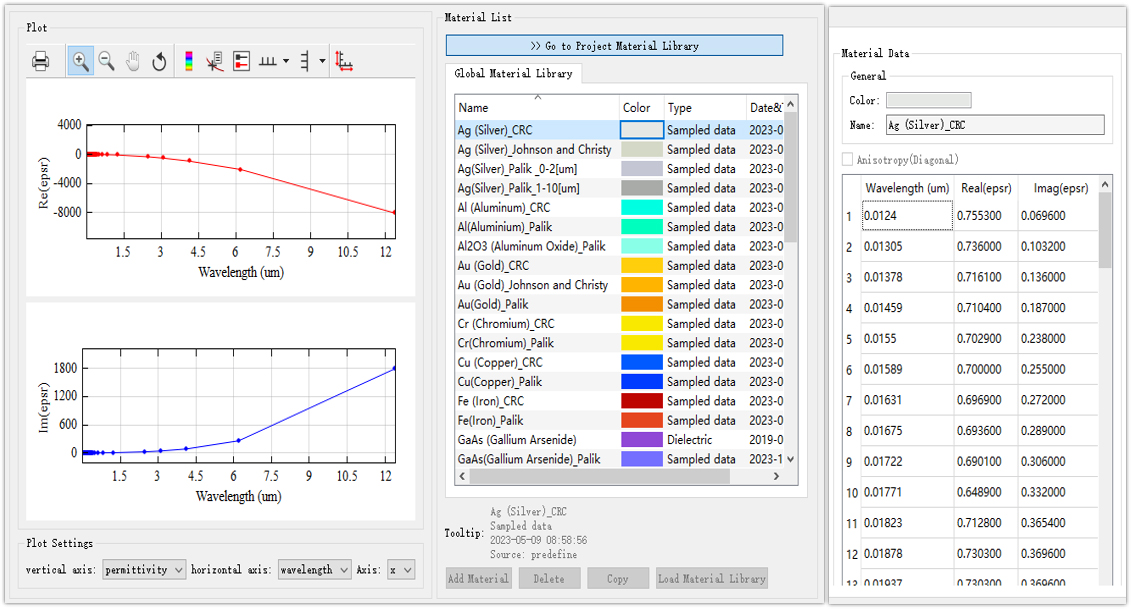
材料属性
- 支持各向异性材料的仿真,允许用户导入自定义的散点材料数据。
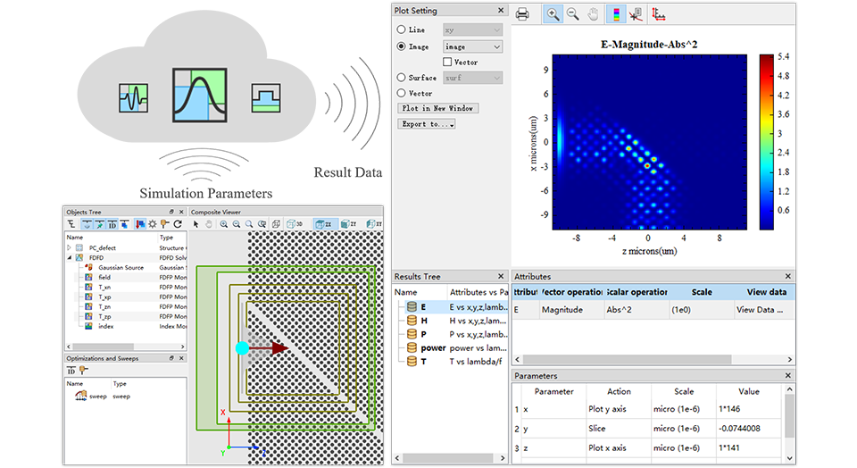
后处理分析
- 功能丰富的后处理分析程序库,包括远场分析、数据展示、电位移矢量分析等。
- 模块化的分析组拥有方便快捷的程序编辑窗口,允许用户灵活地自定义各种分析组。

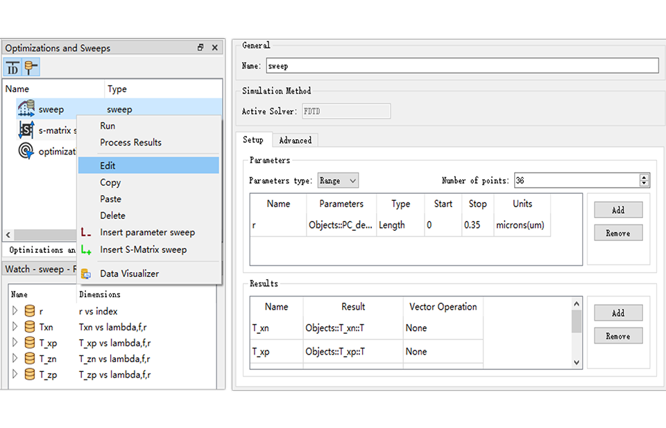
扫描优化
- 支持扫描、优化、S矩阵扫描和嵌套扫描。内置优化算法可自动帮助用户优化器件的设计。
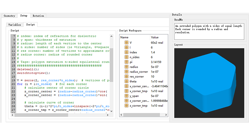
脚本控制
- 脚本功能允许用户操纵仿真中的每一个步骤,实现参数化的构建,为用户提供新的交互体验。
- 软件内置完整的函数库,允许自定义函数,基本满足数学计算的所有需求。
强大的算力
- 在OpenMP、CUDA、MPI、AVX等多种并行计算技术的加持下,算力及运算速度都得到了高效提升。
- 为用户提供云端计算服务,不再局限于本地计算资源。
参考文献
[1] Rumpf, Raymond C et al. “Rigorous electromagnetic analysis of volumetrically complex media using the slice absorption method.” Journal of the Optical Society of America. A, Optics, image science, and vision vol. 24,10 (2007): 3123-34.