Solver

This section describes solvers.

Select the desired solver in the Home tab, click anywhere in the composite view window to add a solver, and edit the solver's properties in the pop-up window. The software offers the following built-in passive solvers:

• FDTD Solver
• FDFD Solver
• FDE Solver

The software allows users to set solvers through scripts. For instructions on using scripts, see Script.

Computational Electromagnetics Algorithm and Solver

Computational Electromagnetics Algorithm

The Preface highlights the irreplaceable role of computational electromagnetics in modern electromagnetic research, and also provides a brief overview of the most popular algorithms currently in use.

The solvers included in the software correspond to three different computational electromagnetics algorithms. Each algorithm is tailored for specific simulation types, offering unique advantages and disadvantages. Therefore, when designing a device, it is important to understand the characteristics of the device as well as the advantages of each algorithm, which facilitates the selection of an appropriate algorithm to achieve the efficient and accurate simulation of the device.

Computational Electromagnetics Algorithm and Solver

The algorithms for computational electromagnetics in this software are integrated within solvers under the Simulation, currently including three types: FDTD, FDFD, and FDE.

Solver and Model

The modeling of devices is independent of simulation solvers, that is, the same device can be solved using different solvers, and vice versa.

Memory Preview before Simulation

After the solver has been added, the software will perform a memory estimation for the entire project, which will assist users in choosing the right computational resources for simulation. Users can view the memory estimation by clicking on 'Check Simulation Memory' in the View tab, as shown in the figure below:

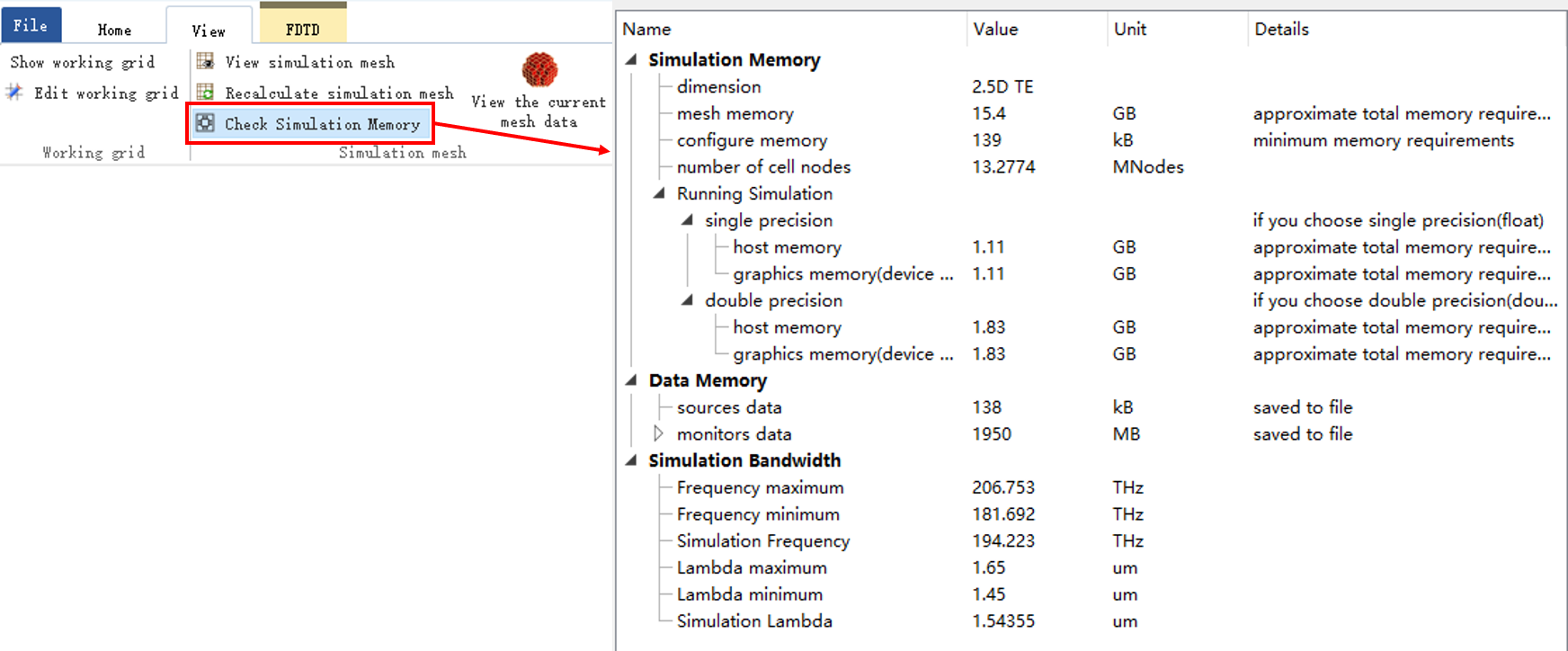
The option Simulation memory indicates the memory required for simulation, Data memory indicates the memory required for recording data, and Simulation bandwidth displays the wavelength and bandwidth calculated during simulation, which does not need to be considered in memory estimation. Mesh memory, Running simulation, and Data memory are important contents for users to consider.

Name	Description
Mesh memory	Represents the memory needed to establish the mesh, which will be released after the mesh is generated;
Running simulation	Require the memory for solver computation;
Single precision/Double precision	Use single-precision or double-precision floating-point data type for data storage and calculations. Users can modify this in the cloud tab;
Host memory/Graphics memory	Indicates the use of CPU/GPU for calculations. Users can refer to the resources selected in the Cloud tab for viewing;
Data memory	Contains the memory required for user to create sources and monitors, where user can view the memory in detail required for each monitor to record data.

When selecting resources for simulation, a comparison should be made between Mesh memory and the sum of the user-selected resources for Running simulation and Data memory. To ensure normal simulation calculation, the selected memory resource must be greater than the larger of these two values above. For example, in the figure above, Mesh memory is 15.4GB, while the memory required for Running simulation calculated by a single precision CPU is 1.11GB. The total is still less than Mesh memory after adding Data memory. Therefore, in this scenario, the memory of the selected computational resource only needs to exceed 15.4GB. For more information on resources, please refer to Computing Resources.

More Information

• Source

  There is no doubt that the source is the most important accessory of the solver.
  For source-excited solvers, users are allowed to select different sources to address various simulation requirements.

• Monitor

  The inspection, display, analysis and export of simulation results must be performed through a monitor.
  The monitor serves as a data collector and has the functionality of analyzing and processing collected data.

• Port

  Certain special features, such as Port, can only be enabled after configuring a specific solver (the Port feature is exclusive to the FDTD solver).