平面光源和高斯光源的设置 #

本节是关于平面光源和高斯光源设置的介绍。

在求解器选项卡中选择Plane或Gaussian后，在复合视图中创建平面光源或高斯光源，并在自动弹出的编辑属性界面中设置参数。

平面光源的设置 #

通用设置 #

• 平面光源
  General标签页的Plane sources选项卡用于设置光源的注入轴和振幅等信息。

Name	Description
Direction	平面光源的注入方向，Forward为正向传播，Backward为反向传播。
Incident axis	下拉选择平面光源的注入轴。

关于平面光源振幅和相移的设置，请参阅光源的通用设置。

• 旋转

关于旋转的设置，请参阅光源的通用设置。

• 多频域

Multi-frequency field属于高级设置，对于一些在仿真带宽内光源变化较小的仿真工程，可以不激活该设置。

Name	Description
Multi-frequency field	多频域，可以求解光源的多个频率在光学器件中的传播特性。此功能推荐应用于宽带时域仿真和光源注入色散材料的仿真工程，特别是涉及到以一定角度注入的情况。
Frequency points	指定将使用多少个频率点来计算光场分布。为了保证精度，频率点至少设置为5。

几何尺寸 #

Geometry标签页用于设置光源的几何范围，请参阅光源的几何尺寸设置。

偏振 #

Polarization标签页用于设置光源偏振，请参阅下文的偏振部分。

波长/频率 #

Wavelength/Frequency标签页用于设置光源的波长/频率信息，请参阅光源的波长/频域设置。

平面光源的更多信息 #

• 如果需要平面光源保持理想的平面波，需要结合实际工程将边界条件设置为周期性边界（Periodic）或布洛赫边界（Bloch）；
• 如果含有平面光源的工程在传播方向上使用PML边界条件，平面光源将在边缘处发生衍射；
• 在宽带仿真中，实际注入角（非零角）随频率的变化而变化，要得到精确的结果，需要对频率或角度进行扫描。

高斯光束的设置 #

基模高斯光束为：

$$E(\rho,z) = \frac{A_0w_0}{w(z)}exp(-\frac{\rho^2}{w^2(z)})exp\{-i\{{k[\frac{\rho^2}{2R(z)}+z]-\Psi(z)}\}\}$$

其中$\rho=\sqrt{x^2+y^2}$，即传播方向为z轴。$|A_0|$为电场的最大幅值，$w(z)$为高斯光束的光斑半径，$w_0$为束腰处的光束半径，也是最小的光斑半径。$R(z)$为波前的曲率半径，$\Psi(z)=tan^{-1}(\cfrac{z}{z_0})$，其中$z_0$称为准直距离，即高斯光束半径扩展到$\sqrt{2}$的距离。

通用设置 #

General标签页用于设置高斯光源相位、振幅和光束轮廓等参数。

光源的注入、旋转和相移 #

Injection选项卡用于设置光源注入轴和注入方向。

Name	Description
Incident axis	高斯光源的注入轴（注入平面的法向）。
Direction	高斯光源的传播方向，Forward为正向传播，Backward为反向传播。

Rotation选项卡是关于旋转的设置，请参阅光源的通用设置。

General选项卡是关于光源注入振幅和相移的设置。请参阅光源的通用设置。

多频域 #

Multi-frequency field属于高级设置，对于一些在仿真带宽内光源变化较小的仿真工程，可以不激活该设置。

Name	Description
Multi-frequency field	多频域，可以求解多个频率的光束在光学器件中的传播特性。此功能推荐应用于宽带仿真和光源注入色散材料的仿真工程，特别是涉及到以一定角度注入的情况。
Frequency points	指定使用多少个频率点来计算光场分布。为了保证精度，频率点至少设置为5。

高斯光束可视化 #

Beam profile选项卡用于绘制高斯光源的场分布。

Name	Description
Current index	注入面的折射率（的最大值），只读参数。
Results	允许用户指定绘制的数据类型，下拉选择Mode fields和Index两种数据类型。
Components	Results选择Mode fields时，分量可选择：E Magnitude，Ex，Ey，Ez，H Magnitude，Hx，Hy，Hz；Results选择Index时，分量可选择：Index_x，Index_y，Index_z。
Scalar	Abs：所选分量的模；Re：所选分量的实数部分；Im：所选分量的虚数部分；Phase：所选分量的辐角。
Regenerate	再次生成图像。
Show/Hide 3D plot	展示/隐藏三维绘图。
Visualize data	打开数据可视化窗口。
Plot in new window	将图像绘制在新的窗口。

高斯光束参数设置 #

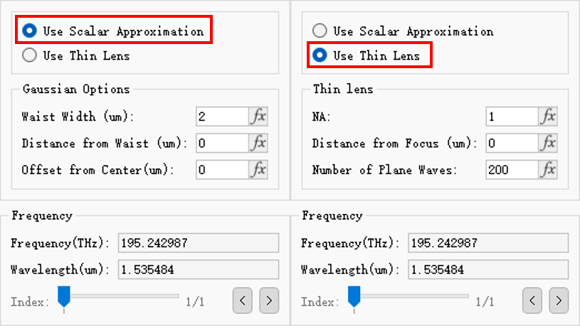
软件提供了两种高斯光源参数设置，一种为使用标量近似的高斯光束（Use scalar approximation），另一种为使用薄透镜聚焦的紧聚焦高斯光束（Use thin lens），后者是一种全矢量光束。在参数设置完成后可以在高斯光束可视化界面当中查看当前光束的场分布。当束腰半径比使用的波长大几倍时，应选择标量近似选项。当束腰半径与波长大致相同时，应使用薄透镜选项。

标量近似的高斯光束 #

Gaussian options选项卡为标量近似的高斯光束参数设置。

Name	Description
Waist width	束腰宽度。
Distance from waist	注入面与束腰的距离。
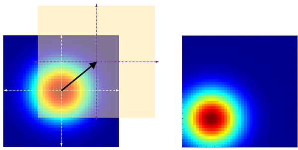
Offset from center	与束腰中心点的横向偏移。

注意：

• 基模高斯光束以光轴为中心的对称分布场，$\rho = \sqrt{x^2 + y^2}$（假设传输方向为$z$）表示注入平面的坐标，参数Offset from center是指注入光场的中心与高斯光束的中心的偏离；
• 基模高斯光束适用于满足傍轴条件的模型，对于非傍轴情况不能准确描述。傍轴近似要求满足$\lambda << w_0$，在仿真中至少是$\lambda \approx w_0$。

紧聚焦高斯光束 #

以下为使用薄透镜聚焦的紧聚焦高斯光束，Thin lens选项卡设置透镜相关参数。

Name	Description
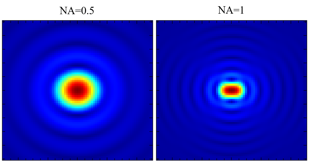
NA	薄透镜的数值孔径，即为$n*sinA$，$n$为光源所在位置的折射率，A为半角宽度，下图展示了不同数值孔径下的高斯光源场分布。
Distance from focus (um)	注入平面与透镜焦点的距离，正数表示发散光束，负数表示会聚光束。
Number of plane waves	构建光束的平面波数，数字越大，光束轮廓越准确，但同时也会增加计算时间。

几何尺寸 #

Geometry标签页用于设置光源的几何范围，请参阅光源的几何尺寸设置。

偏振 #

Polarization标签页用于设置光源偏振，请参阅下文偏振部分。

波长/频率 #

Wavelength/Frequency标签页用于设置光源的波长/频率信息，请参阅光源的波长/频率设置。

偏振 #

局域偏振和全局偏振 #

偏振是对于平面光源定义的，在FDTD求解器中，支持对高斯光源的光场定义复杂的偏振。

对于平面光源和高斯光源，支持的偏振类型有：

• 全局偏振（Global polarization），即注入平面每个点的偏振特性相同，使用一个琼斯矢量（Jones vector）即可表示，软件提供了典型的如：线性偏振、左（右）旋圆偏振、左（右）旋椭圆偏振等；
• 局域偏振（Local polarization），即注入平面每个点的偏振特性不同，软件提供了典型的偏振特性：径向偏振、角向偏振、涡旋偏振、任意偏振；
• 用户自定义偏振（User‘s polarization）。

偏振的设置 #

Name	Description
Linearly polarization(θ)	在线性偏振中，定义线性偏振的偏振角。
Elliptically orientation angle	在左（右）旋椭圆偏振中，定义椭圆方位角。
Elliptically U	在左（右）旋椭圆偏振中，定义椭圆第一个轴长 U。
Elliptically V	在左（右）旋椭圆偏振中，定义椭圆第二个轴长 V。
Order 1	在径向/角向/涡旋偏振中，定义第一个径向阶数。
Order 2	在径向/角向/涡旋偏振中，定义第二个径向阶数。

案例：定义圆偏振 #

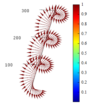
定义左旋圆偏振的平面波：

使用Vector绘图方式绘制传输方向上光的电场矢量，如下图所示，电场矢量在传输方向上呈现明显的圆形轨迹。