
/
导入光源的设置
用户自定义光源导入光源非傍轴高斯源导入
导入光源的设置 #
本节是关于导入光源设置的介绍。
导入光源提供了更多的选择空间,这里介绍了导入光源的相关设置。
在求解器选项卡中选择Import后,在复合视图中创建导入光源,并在自动弹出的编辑属性界面中设置参数。
导入光源的设置 #
通用设置 #
General source 用于设置光源的注入轴和振幅等信息。
| Name | Description |
|---|---|
| Incident axis | 下拉选择导入光源的注入轴。 |
| Direction | 导入光源的注入方向,Forward为正向传播,Backward为反向传播。 |
关于导入光源振幅、相移和旋转的设置,请参阅光源的通用设置。
Import data选项卡用于设置导入数据。
| Name | Description |
|---|---|
| Spatial position | 导入数据的空间位置,可选择网格边界的中心,即:Yee-cell,或网格的交点,即:Nearest mesh cell。 |
| Finite-difference type | 有限差分的类型,分为:中心有限差分(Central finite difference)和基于Yee元胞的有限差分(Yeecell-based finite difference)。 |
| Imported data from path | 导入路径,只读参数。 |
| Visualize data | 打开可视化窗口。 |
| Import source | 进入选择导入文件界面。 |
几何尺寸 #
Gemetry标签页用于设置光源的几何尺寸,请参阅光源的几何尺寸设置。
波长/频率 #
Wavelength/Frequency标签页用于设置光源的波长/频率信息,请参阅光源的波长/频率设置。
案例 #
导入源的核心问题是场数据的构造。软件要求以固定的数据集格式将电磁场的数据传递给导入光源。
我们将展示如何使用导入光源,在本案例中,首先构建一个以z轴入射的高斯光源数据集,脚本为:
# Define parameters;incident axis is Z
points = 201;
x = linspace(-5e-6, 5e-6, points);
y = linspace(-4e-6, 4e-6, points);
z = -4e-6;
lambda = 0.5e-6;
f = c/lambda;
index = 1;

# Calculate field components using Gaussian formula
[x0,y0] = meshgrid(x,y);
w0 = 1e-6;
f_a = exp(-((x0/w0).^2 + (y0/w0).^2));
f_a = f_a.';
Ex = f_a;
Ey = zeros(points, points);
Ez = zeros(points, points);
Hx = zeros(points, points);
Hy = f_a*sqrt(eps0/mu0);
Hz = zeros(points, points);

# Create EH dataset
Gaussian_fields = matrixdataset('fields');
Gaussian_fields.addparameter('x', x);
Gaussian_fields.addparameter('y', y);
Gaussian_fields.addparameter('z', z);
Gaussian_fields.addparameter('lambda', lambda, 'f', f);
Gaussian_fields.addattribute('E', Ex, Ey, Ez);
Gaussian_fields.addattribute('H', Hx, Hy, Hz);
Gaussian_fields.setparameterunit('x','length');
Gaussian_fields.setparameterunit('y','length');
Gaussian_fields.setparameterunit('z','length');
Gaussian_fields.setparameterunit('lambda','length');
Gaussian_fields.setparameterunit('f', 'frequency');

# Save the dataset as a .mat file
savematlabmatfile('Gaussian_fields.mat', Gaussian_fields);
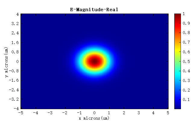
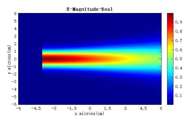
将上述脚本生成的数据集Gaussian_fields.mat导入Import source中,运行FDTD仿真,在监视器中查看传输场,其结果如下所示:
| Import-E magnitude | Transmission field-E magnitude |
|---|---|
 |
 |
因此,用户可以根据自己的需求,将任意场数据按照上述数据集格式导入,从而形成自定义的导入光源。