Mesh Setting

This section describes mesh setting in solver.

Mesh is one of the most important settings in a solver and its partitioning has a direct impact on simulation accuracy and efficiency.

Mesh Type

There are several mesh types:

Name	Description
Uniform	It contains mesh cells in the same size, can be partitioned by a simple and intuitive method, and suitable for most simulation scenarios.
Semi-auto nonuniform	The mesh size can be defined by users in the simulation region to meet specific simulation requirements.
Auto nonuniform	The nonuniform mesh can be automatically generated based on the user-defined mesh accuracy level to improve simulation accuracy and computational efficiency.

For Auto nonuniform mesh, Accuracy level shall be set up to select the mesh accuracy. The mesh accuracy is classified into 10 levels, with level 1 corresponding to the coarsest and level 10 corresponding to the finest. The expression is

$N=\cfrac{\lambda_0}{n \Delta}$

where $\lambda_0$ is the wavelength in vacuum, n is the refractive index of the material, and $\Delta$ is the grid size. The equation indicates that the mesh accuracy is related to wavelength and material refractive index. For instance, in a vacuum, at Accuracy Level 1, 6 grids are divided within the spatial extent of a single wavelength; at Level 2, there are 10 grids. The grid count increases by increments of 4. The meshing algorithm will use a smaller mesh in high index materials. A finer mesh minimizes the effects of numerical dispersion, but significantly elevates the need for computational speed and resources. It is recommended that users make a tradeoff to select an appropriate mesh accuracy level to achieve the best outcomes according to specific project requirements and available computational resources. For most applications, a setting of between 2 and 5 is sufficiently accurate.

Mesh Refinement

To improve the mesh accuracy and precision of electromagnetic simulation, we can increase mesh density or adjust mesh size to enhance the discretization quality of the simulation region. Currently, there are two mesh refinement methods built in the software.

• Staircase: When a single mesh cell contains a plurality of materials, the staircase mesh refinement method fills the entire cell with a single material.
• Conformal: The conformal mesh refinement method calculates the average permittivity of subcells on the boundary of the curved structure, so as to obtain a higher interface resolution. The conformal mesh refinement method can achieve accurate results even with a relatively coarse mesh.

The available mesh refinement methods built in the software comprise the following:

Name	Description
Staircase	Based on whether the center of the Yee mesh is in the structure, assign a single material property to the mesh, so that the resulting discrete structure cannot show the structure changes in the mesh.
Conformal variant VP-EP	Based on mesh at material boundary, the effective permittivity can be calculated by using proportions of different materials and the normal direction relation of electric field with respect to the interface of structure.
Conformal variant V-EP	The effective permittivity can be obtained by calculating the simple volume average of different materials in the same mesh.
Conformal variant Yu Mittra 1	Applicable to metallic materials or PEC materials. The Maxwell equation of the mesh near the conductor surface is modified by using the loop integration in which the internal electric field of the ideal conductor is 0.
Conformal variant Yu Mittra 2	Located on the surface of dielectric or non-metallic materials, with effective permittivity obtained by weighted average of the lengths occupied by different dielectric materials on the corresponding edge of the Yee mesh.

Mesh refinement subcells:

Name

Description

Mesh refinement subcells

Except for the Staircase setting where this parameter does not exist, all the other types of mesh refinement have this parameter. It is used to specify how many subcells the current single mesh will be divided into for calculating the effective permittivity. In 2D simulation, a single mesh is subdivided into $N\times N$ subcells, while in 3D simulation, a single mesh is subdivided into $N\times N\times N$ subcells, where N is the Mesh refinement subcells value specified by the user.

Mesh Definition Type

The related setting for Mesh definition type are displayed when the mesh type is set to Uniform and Semi-auto nonuniform.

Mesh definition type:

Name	Description
Mesh size	Mesh size.
Number of mesh cells	Total number of mesh cells in the simulation region along a single direction (X/Y/Z).
Mesh cells per wavelength	Number of mesh cells per unit wavelength (or number of sampling points per wavelength).
Reference wavelength	Enabled in Mesh cells per wavelength type, defining the reference wavelength corresponding to the mesh.
Cells Z/X/Y	Enabled in Mesh cells per wavelength type, defining the number of mesh cells corresponding to the reference wavelength in the Z/X/Y direction.
dz/dx/dy	Enabled in Number of mesh cells type, defining the spatial interval in the Z/X/Y direction.
Cells z/x/y	Enabled in Mesh size type, defining the total number of mesh cells in the simulation region along the Z/X/Y direction.

Time Step Size

Time step size:

Name	Description
Stability factor	The ratio between the maximum allowable step size of each time step and the actual time step size used. This parameter is used to determine if the time step size is small enough to maintain numerical stability and accuracy, with a default value of 0.99.
dt	Time step size, a read-only parameter.

Minimum Mesh Size

Minimum mesh size setting:

Name	Description
Min mesh size setting	Define the minimum size of a single mesh cell; in general, a smaller minimum mesh size can provide finer resolution, but requires more computational resources.

More Information

Mesh Order

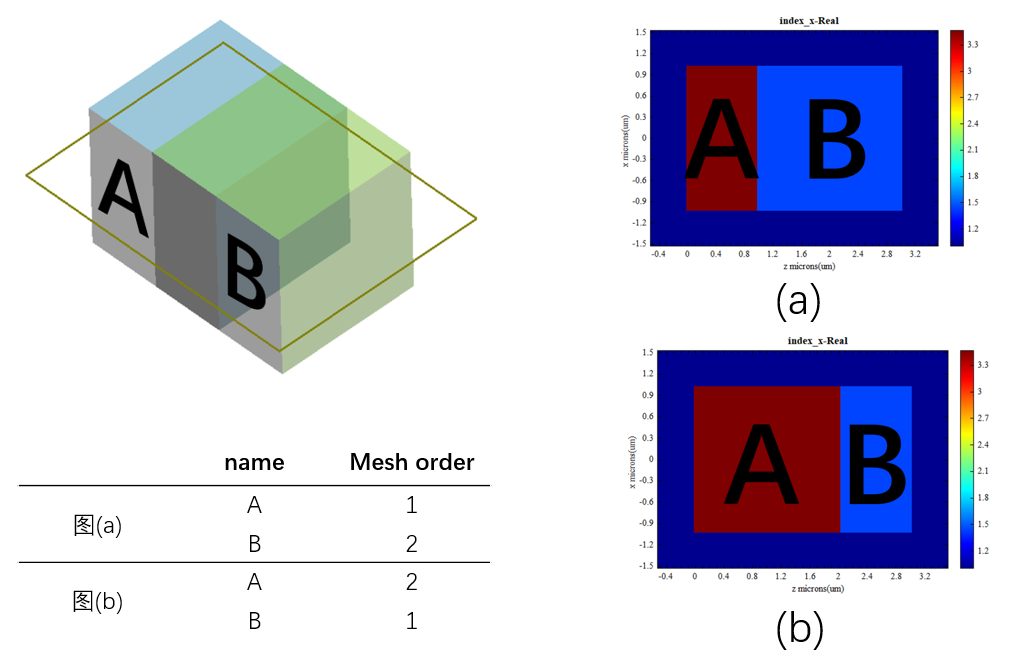
Mesh order is a structural property used to set the order in which meshes are created.

When structures overlap in space, the selection of materials for the overlapping region can be controlled by setting the Mesh order (the larger the Mesh order, the higher the material grade). The specific setting steps are as follows: select a structure, right-click to open the Edit properties window, switch to the Material tab, tick Override mesh order (inactivated by default), and set the number of levels for Mesh order.

By modifying the Mesh order for structure A and structure B, the material selection for the intersecting space is specified, as shown in the figure below.

Case Study: Combination Effect of Different Mesh Types and Refinement Methods

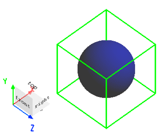
Create a simple model: dielectric sphere project with $\widetilde{N} = 3.472$.

Set up using different mesh types and refinement methods, as shown in the table below:

Name	Mesh type	Mesh refinement	More
$(a)$	Uniform	Staircase	A simpler mesh setting, with higher partitioning efficiency.
$(b)$	Auto nonuniform	Staircase	Efficient and accurate partitioning.
$(c)$	Uniform	Conformal variant VP-EP	Better modeling effect for devices sensitive to boundaries.

Use View the current material data to see the created results (for a combination of other mesh types and refinement methods, please try it yourself):

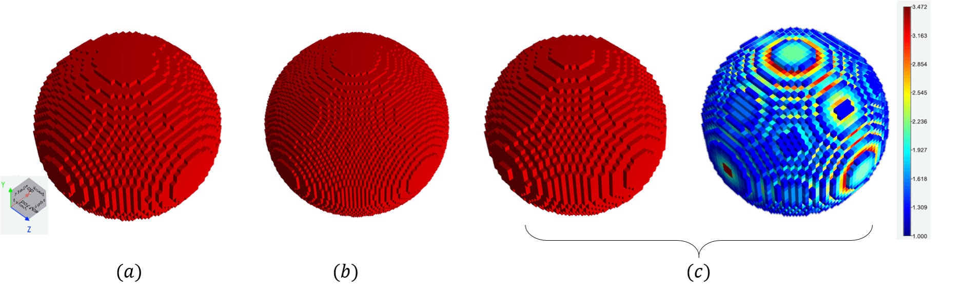
Add Index monitor to view the material distribution in the central cross-section.

Related Publications

[1] Yu W, Mittra R. A conformal finite difference time domain technique for modeling curved dielectric surfaces[J]. IEEE Microwave and Wireless Components Letters, 2001, 11(1): 25-27.
[2] Taflove A, Hagness S C, Piket-May M. Computational electromagnetics: the finite-difference time-domain method[J]. The Electrical Engineering Handbook, 2005, 3: 629-670.
[3] Zhao Y, Hao Y. Finite-difference time-domain study of guided modes in nano-plasmonic waveguides[J]. IEEE transactions on antennas and propagation, 2007, 55(11): 3070-3077.
[4] Mohammadi A, Nadgaran H, Agio M. Contour-path effective permittivities for the two-dimensional finite-difference time-domain method[J]. Optics express, 2005, 13(25): 10367-10381.