FDFP监视器的设置
FDFP监视器的设置 #
本节是关于频域场功率(Frequency domain field and power, FDFP)监视器设置的介绍。
FDFP监视器用于计算指定几何空间中的频域电磁场的数据。
在求解器选项卡中选择FDFP monitor,在复合视图中单击,并在自动弹出的属性编辑界面设置相关参数,以完成FDFP监视器的创建。
FDFP监视器计算处理 #
时域、空域、频域定义的物理量由傅里叶变换联系在一起,而FDFP监视器可以将时域场信号转换为频域场信号。因此,FDFP监视器不仅能够记录数据,还能够计算处理数据。
电场和磁场 #
电场 #
FDFP监视器返回的频域电场公式如下:
E(ω)=∫E(t)e−iωtdt
E(t)为时域电场,e−iωt为复指数函数,t为时间。
磁场 #
FDFP监视器返回的频域磁场公式如下:
H(ω)=∫H(t)e−iωtdt
H(t)为时域磁场,e−iωt为复指数函数,t为时间。
能量、功率、透过率 #
坡印廷矢量 #
FDFP监视器的坡印廷矢量计算公式如下:
P(ω)=E(ω)×H(ω)∗
E(ω)为频域电场, H(ω)∗ 为频域磁场的共轭复数。
功率 #
FDFP监视器的功率计算公式如下:
power=21∫P(ω)⋅ds
P(ω)为坡印廷矢量,ds为表面法向。
透射率 #
FDFP监视器的透射率计算公式如下:
T(ω)=sourcepower(ω)0.5∫Re(P(ω))⋅ds
P(ω)为坡印廷矢量,sourcepower(ω)为入射功率,ds为表面法向。
FDFP监视器的设置 #
通用设置 #
General标签页是关于FDFP监视器的通用设置。
数据监测 #
| Name | Description |
|---|---|
| Data type | 记录数据的数据类型,默认为Frequency-domain,只读参数。 |
| Spatial interpolation | 下拉选择空间插值的类型:None:不进行任何空间插值操作,记录网格内不同位置的电磁场分量;Mesh cell:电场和磁场的每个分量被记录在网格的不同位置,当用户选择Mesh cell插值类型后,电磁场的分量就会被插值到最近的网格单元边界上。这种插值方式是将场分量内插到网格的同一位置,以确保坡印廷矢量的正确计算。 |
| Record data in PML | 记录PML区域内的数据,此项为高级设置,默认不勾选。 |
分量 #
| Name | Description |
|---|---|
| Components | 电磁场分量:Ex、Ey、Ez;Hx、Hy、Hz;坡印廷矢量:Px、Py、Pz。 |
频率采样 #
| Name | Description |
|---|---|
| Min sampling per cycle | 每个周期的最小采样数;用于设置每个周期内采样的点数,默认值为2。 |
| Desired sampling | 期望采样;用于控制采样密度的参数,指定仿真过程中对场进行采样的间隔或步长。 |
| Nyquist limit | 奈奎斯特采样极限;为了能够准确地重构一个连续时间信号,必须以不低于待分析信号最高频率两倍的采样率对信号进行采样。 |
| Sampling frequency | 采样频率;表示单位时间内对连续信号进行采样的次数。采样频率应不低于待分析信号最高频率的两倍,以遵循奈奎斯特极限的要求。 |
| Sample time(per # of dt) | 采样时间;在仿真过程中进行采样的时间间隔,即在多少个时间步长之后对场进行一次采样。 |
空间采样 #
| Name | Description |
|---|---|
| Per # of dx/dy/dz | 仿真过程中沿着X/Y/Z方向采样的间隔,即在多少个离散化步长之后进行一次采样。 |
几何尺寸 #
Geometry是FDFP监视器几何尺寸设置标签页。详情请参阅监视器的几何尺寸设置。
波长/频率 #
频率设置 #
Frequency settings标签页用于设置FDFP监视器的带宽范围和频点数。
- 基于光源的设置
勾选Base on source setting后,该标签页的波长/频率范围显示光源的波长/频率范围,且波长/频率范围的设置选项卡为只读状态。
取消勾选Base on source setting后,该标签页的波长/频率范围允许自定义。
- 简化编辑
Edit simplified settings为监视器自定义波长范围的简化编辑方式。
- 复杂编辑
Edit complicated settings为监视器自定义波长/频率范围的复杂编辑方式。
切趾 #
傅里叶变换是研究整个时域和频域的关系。在仿真过程中无法对无限长的信号进行测量和运算,而是取其有限的时间片段进行分析。可采用不同的窗口函数对信号进行切趾,利用窗口函数将采样区域边缘的信号平滑地降至零。
| Name | Description |
|---|---|
| Apodization type | 下拉选择切趾类型。 |
| Apodization function | 下拉选择切趾窗函数类型。 |
| Apodization center | 窗函数中心位置,即时域信号开始衰减的位置。 |
| Apodization time width | 控制窗函数在时间域上的宽度,即窗函数从开始生效到完全衰减所经过的时间。较短的时域宽度会导致更快的衰减速度,而较长的时域宽度则会产生更缓慢的衰减。 |
切趾类型可分为以下三种:
| Name | Description |
|---|---|
| None | 不对时域信号切趾。 |
| Full | 时域完整的窗口函数,时域信号转换为频率后,仅窗口处数据会保留。 |
| Start | 从时域信号的起始位置处进行衰减,过滤前端的时域数据。 |
| End | 从时域信号的结束位置处进行衰减,过滤仿真后端的时域数据。 |
软件内置的窗口函数类型有以下九种,每种窗口函数都有不同的特性,用户可以根据实际需求选择合适的窗函数:
Gaussian:在时域上呈现出高斯分布的形状,具有平滑的衰减特性。高斯窗口函数在频域上的主瓣较宽,因此频率分辨力低。其表达式为:
ω(t)=e−2σ2t2
σ是控制窗口带宽的标准差参数,t是时间。
Bartlett:在时域上呈三角形,具有平滑的衰减特性。它的幅度从窗口中心向两端逐渐减小,类似于一个对称的三角形Bartlett窗函数。在频域上具有较宽的主瓣和相对较高的旁瓣功率,因此在需要较好的频谱分辨率和较小的旁瓣泄漏时,可能需要考虑其他类型的窗口函数,如Hanning窗、Hamming窗、Blackman窗等。其表达式为:
ω(t)=1−T∣t∣
t是时间,T是窗口的时域宽度。
Blackman:在时域上呈平滑的衰减特性,包含了一个主要的余弦项和一个次要的余弦项,这使得它在频域上能够提供更好的旁瓣抑制和频谱分辨率。其表达式为:
ω(t)=0.42−0.5cos(T2πt)+0.08cos(T4πt)
t是时间,T是窗口的时域宽度。
Connes:在时域上振幅分布呈平滑的曲线形状。与其他窗口函数相比,它在起始和结束位置处的振幅衰减更加缓慢。其表达式为:
ω(t)=(1−(2T)2t2)2
t是时间,T是窗口的时域宽度。
Cosine:在时域上振幅分布呈周期性变化,从最小值到最大值,再回到最小值。这种周期性变化使得时域信号的振幅均匀分布。其表达式为:
ω(t)=cos(Tπt)
t是时间,T是窗口的时域宽度。
Hanning:在时域上呈平滑的衰减特性,类似于余弦波形。Hanning窗口函数的优点是平滑衰减的形状有助于减小频谱泄漏,提供较好的频谱分辨率。缺点是在时域上的平滑衰减特性会导致频域上的主瓣宽度增加。其表达式为:
ω(t)=0.5−0.5cos(T2πt)
t是时间,T是窗口的时域宽度。
Hamming:在时域上呈现出平滑的衰减特性,类似于余弦波形,与Hanning窗函数类似。Hamming窗函数具有较低的旁瓣功率和频谱泄漏。与Hanning窗函数相比,Hamming窗函数在窗口两端的值衰减得更快,因此在频谱分析中能够提供更好的旁瓣抑制能力,但同时也会导致较宽的主瓣。其表达式为:
ω(t)=0.54−0.46cos(T2πt)
t是时间,T是窗口的时域宽度。
Welch:在时域上呈类似于抛物线的形状,具有较好的旁瓣抑制能力。它与Bartlett窗函数类似,但在窗口两端的衰减速率更快。其表达式为:
ω(t)=1−(2T)2t2
t是时间,T是窗口的时域宽度。
Uniform:矩形窗口函数;窗口内部取值为常数1,窗口外部取值为0。该函数的优点是主瓣比较集中,缺点是没有平滑衰减特性,具有较大的频谱泄漏和旁瓣功率。其表达式为:
ω(t)={10−2T≤t≤2Totherwise
t是时间,T是窗口的时域宽度。
模式扩展 #
Mode expansion为FDFP监视器的模式扩展的设置,具体的设置细节请参阅FDFP监视器模式扩展。
数据可视化 #
使用FDFP监视器保存由时域仿真计算得到的频域场数据集,返回的结果数据包括:
- E:电场与频率(波长)的关系;
- H:磁场与频率(波长)的关系;
- P:坡印亭矢量与频率(波长)的关系;
- Power:功率与频率(波长)的关系;
- T:透射率与频率(波长)的关系。
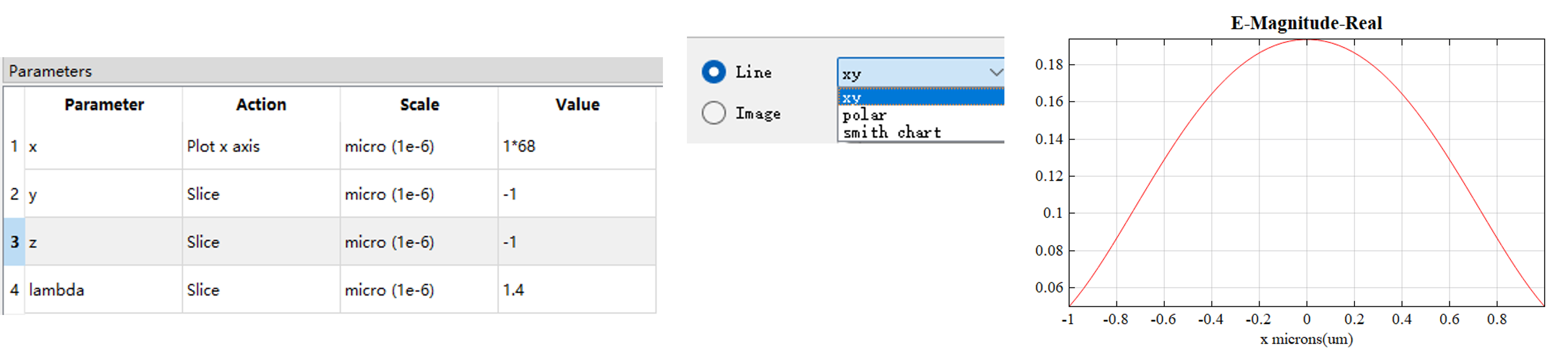
在FDFP监视器的可视化窗口中,可查看该频域场分布,操作如下图:

在数据可视化界面,可实现对数据的选取、绘制和保存等操作,详情请参阅数据可视化。
比如查看Ex分量的实部,Attributes的设置和结果如图所示:
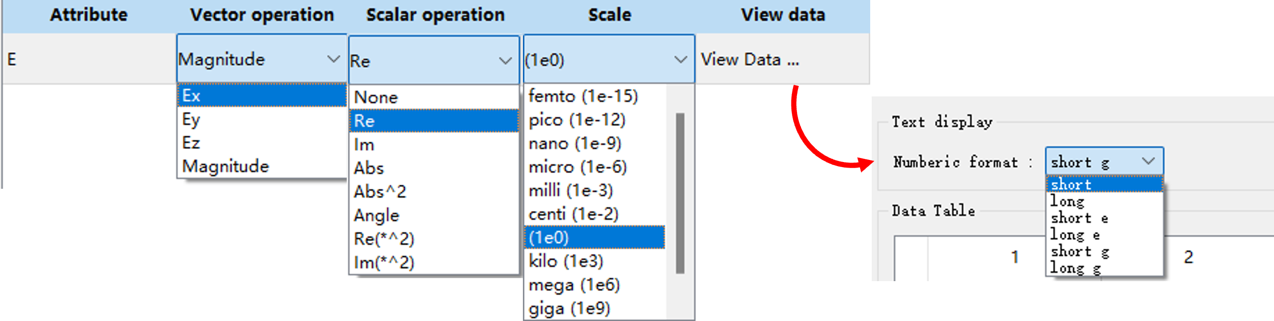
将一维数据集绘制为1D线图: