边界条件设置
边界条件设置 #
本节是关于求解器边界条件的介绍。
边界条件是求解器重要的设置之一。选择合适的边界条件,可以很大程度上提高仿真效率和准确性。
边界条件 #
边界条件的类型包括:
| Name | Description |
|---|---|
| PML | 完美匹配层(Perfect match layer);PML边界条件可以有效地吸收从计算区域边界入射或反射的电磁波,防止波的反射。 |
| Periodic | 周期边界;通过模拟一个单元来计算整个周期性系统的响应。 |
| Bloch | 布洛赫边界;当结构具有周期性,适用于周期性光源在单波长指定入射角入射时。 |
| PEC | 完美电导边界(Perfect electrical conductor);平行于PEC边界的电场分量为零;垂直于 PEC 边界的磁场分量也为零。PEC边界具有全反射特性。 |
| PMC | 完美磁导边界(Perfect magnetic conductor);平行于PMC边界的磁场分量为零;垂直于PMC边界的电场分量也为零。PMC边界具有全反射特性。 |
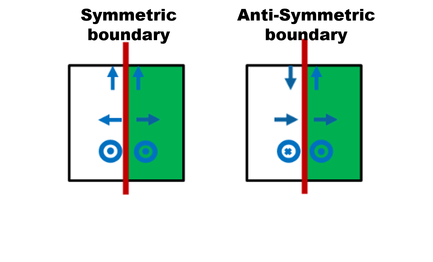
| Symmetric / Anti-symmetric | 对称/反对称边界;当设置对称/反对称边界时,仿真区域内电磁场也是符合对称/反对称设置要求的。 |
PML #
PML的效果 #
这里展示PML的实际效果。
使用FDFP监视器(FDFP monitor),记录穿越PML边界的场值随距离的衰减趋势。
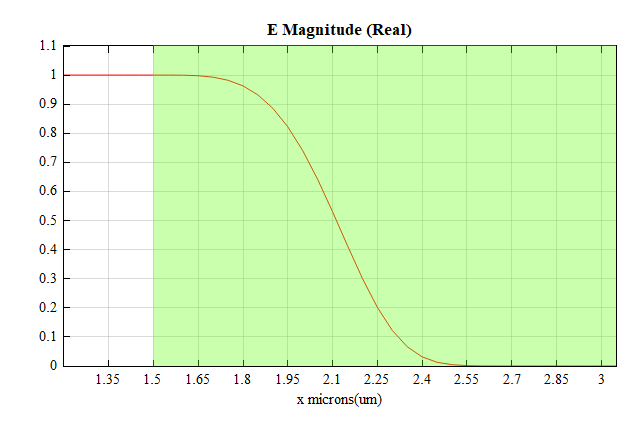
可见,光入射到PML以后,随着PML的逐层吸收,入射光迅速衰减到可以被忽略的量级。
PML和结构 #
软件使用拉伸型PML,对于穿越PML边界的结构请参阅结构页面的边界部分。
在FDTD属性边界条件选项卡中包含Extend Structure through PML的选项,如下图所示,该选项为默认勾选。
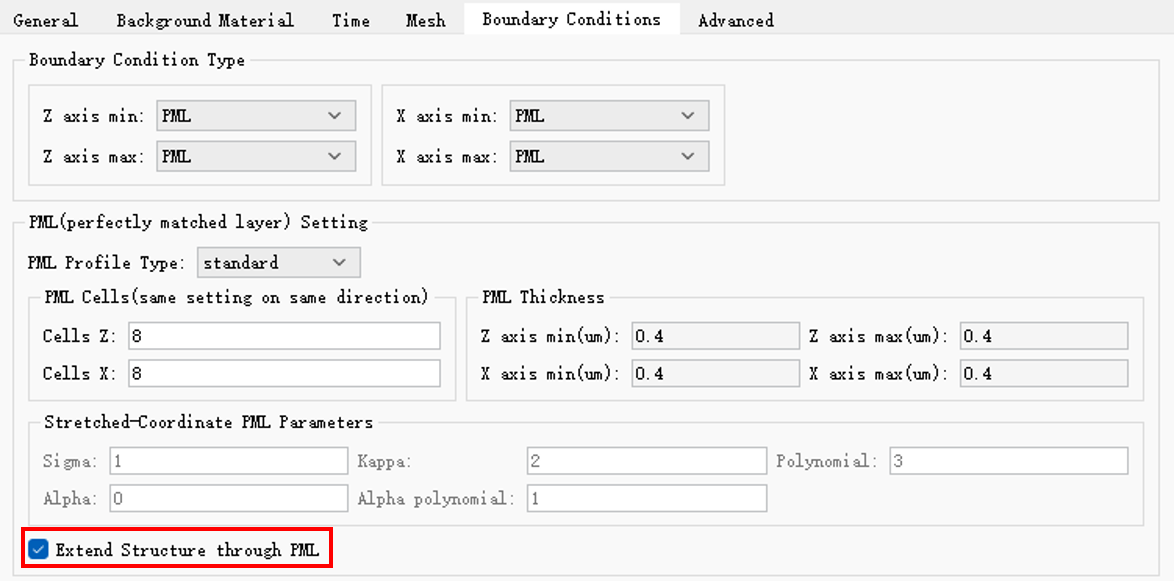
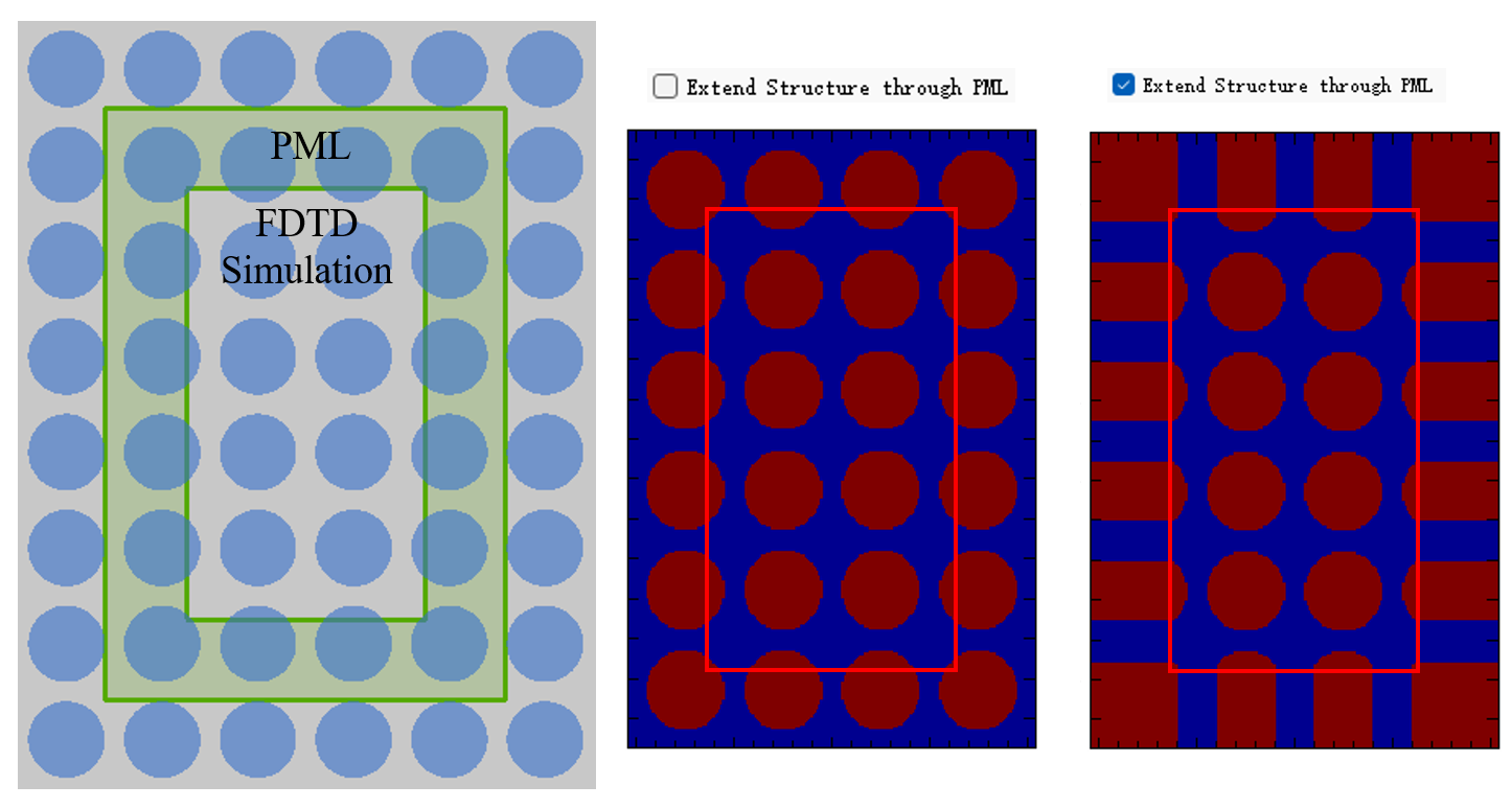
当勾选该选项时,软件将在垂直于边界的方向上自动拓展与PML内边界接触的结构。对于多层材料的平板结构,勾选该选项将减少仿真区域和边界之间的反射,从而增强PML的吸收性能。因此,我们建议用户勾选此选项,以降低杂散光的反射。

值得注意的是,对于光子晶体等周期结构,正确做法是取消勾选该选项,以避免将接触内边界的晶体结构拓展,从而保持光子晶体的周期性。
PML和光源、监视器 #
允许光源和监视器的空间尺寸超出仿真区域,但注意:
-
默认情况下,光源超出仿真区域部分无效;
-
默认情况下,监视器超出仿真区域部分不记录数据;
-
在监视器中,存在记录PML场的设置:Record data in PML。
PML的配置类型 #
软件内置了三种预定义的PML配置类型,用于调整和优化吸收层的性能,用户可通过PML配置类型(PML profile type)下拉菜单中选择PML配置类型。
| Name | Description |
|---|---|
| Standard | 标准配置;该配置类型以相对较少的层数提供良好的整体吸收,建议优先考虑该选项。标准配置适用于结构未穿过PML区域的仿真工程。 |
| Stabilized | 稳定配置;当材料边界穿过PML层时或者光源大角度入射到PML层时,有可能出现数值不稳定性。使用稳定性配置可以避免光在PML层内出现发散。稳定配置主要通过调节PML的参数和增加PML层数来增强稳定性,需要较多的PML层数才能达到较好的吸收效果,同时会增加计算的复杂性和资源需求。 |
| Custom | 自定义配置;允许用户对PML参数值进行输入,自定义配置的默认值是标准配置的参数值。建议用户在充分理解PML原理后,再尝试进行该项设置。 |
PML的设置 #
对于自定义配置(Custom)类型,允许用户自定义的参数有:
| Name | Description |
|---|---|
| Cells Z/X/Y | PML单元个数。 |
| Sigma | PML层的电导率;用于调整PML层对电磁波的吸收能力。 |
| Alpha | PML层损耗系数;用于降低PML表面对于低频率信号的反射。 |
| Kappa | 无单位。 |
| Polynomial | 使用多项式函数来描述 Kappa 和 Sigma 的变化。 |
| Alpha polynomial | 使用多项式函数来描述 Alpha 的变化。 |
对于标准配置(Standard)或者稳定配置(Stabilized)类型,唯一允许用户自定义的参数是:
| Name | Description |
|---|---|
| Cells Z/X/Y | PML单元个数。 |
周期边界 #
-
周期边界或布洛赫边界同一方向(X/Y/Z)的上下边界条件必须保持一致。
-
使用周期性边界条件,工程中的一切都必须是周期性的,包括结构和电磁场。请注意以下两种情况不支持使用周期边界条件:
-
以一定角度入射的平面波通过周期性结构,在这种情况下,光源具有相移,需要使用 Bloch 边界;
-
周期结构由单个非相干的偶极子光源激发,在这种情况下,工程不是周期性的。
-
布洛赫边界 #
布洛赫边界条件(Bloch)主要应用于以一定角度入射的平面波通过周期性结构的工程。布洛赫边界是对模拟区域一个边界的场进行相位矫正后注入至另一个边界。
用公式表示为:
Exmax=e−iax kxExmin
Exmax=eia∗x k∗xExmin
其中k∗x为布洛赫波矢,a∗x为平移的晶格矢量。
在FDTD中,使用Sine-cosine方法实现单频点的布洛赫边界条件,对于宽带仿真,需要配合软件内置的扫描功能才能得到正确结果,详见扫描。
对于布洛赫边界,默认勾选Using source angle,基于光源的角度计算布洛赫波矢,若取消勾选,则需要用户自定义布洛赫波矢。
| Name | Description |
|---|---|
| kx/ky/kz | 波矢K沿着 x/y/z 方向的分量。 |
在分析能带的问题中,扫描频率和布洛赫波矢是相互配合且必不可少的设置。
PEC #
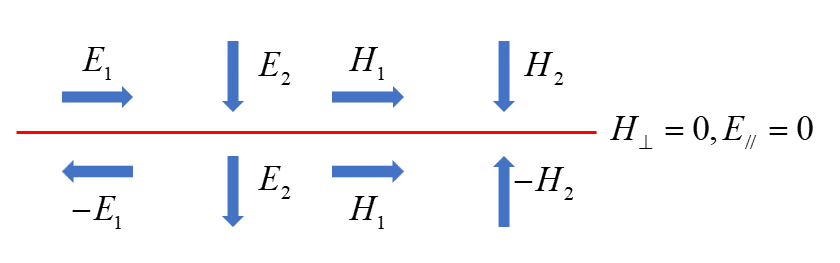
PEC边界条件,平行于PEC边界的电场分量为零,垂直于PEC边界的磁场分量也为零。即:
PMC #
PMC边界条件,平行于PMC边界的磁场分量为零,垂直于PMC边界的电场分量也为零。即:
对称/反对称 #
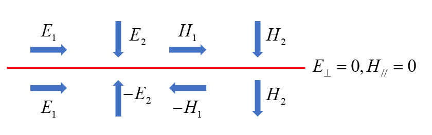
对称/反对称边界的电磁场 #
- 对于对称/反对称边界中的电场,有:
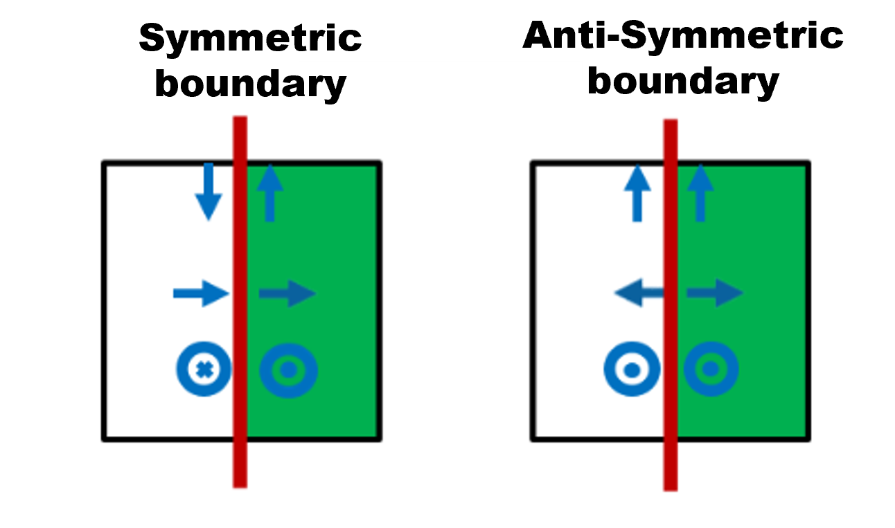
- 对于对称/反对称边界中的磁场,有:
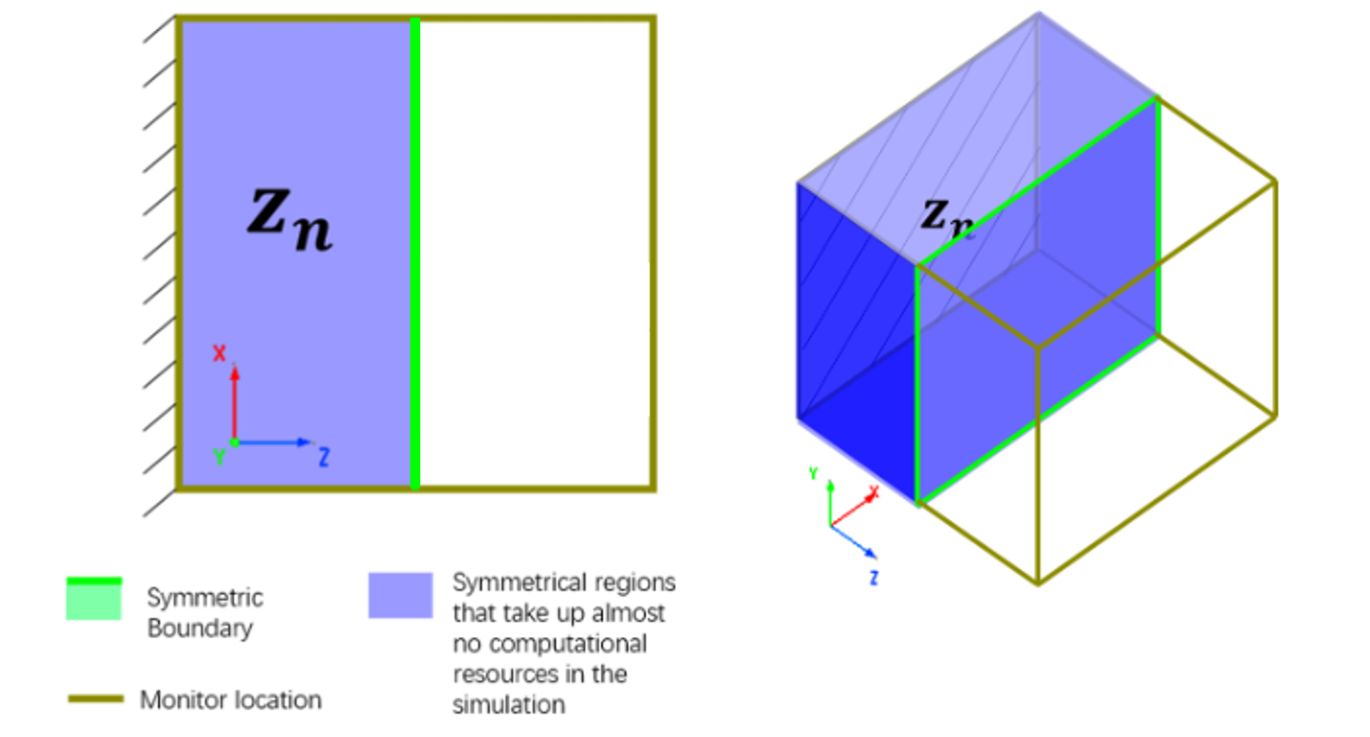
对称/反对称边界的设置 #
对称/反对称边界,不仅要求物理结构(包括几何结构和材料)对称,而且要求光源的场分布对称。利用这种对称性,可以将计算空间减少一半(每个方向),能够很大程度的加快仿真速度。
对称/反对称的使用技巧 #
- 对于器件而言,需要满足结构和仿真区域对称;
- 将光源放置在恰当的位置,以满足对称/反对称边界的要求。
周期边界和对称/反对称边界 #
对于周期边界,当仿真工程满足对称条件时,允许使用对称/反对称边界等效替换,以减少仿真计算量。