函数
The section introduces the function, including user-defined functions and advanced built-in analysis functions used to process the complicated physical problems.
User functions #
Script library allows users to define their own script functions to implement advanced operations conveniently and make code more reusable, maintainable, and understandable. Furthermore, script library also provides various useful operations on user-defined functions.
user function #
Description
Use the function command to create your own script functions, which allows you to write more reusable, maintainable, and understandable code. User-defined functions support arbitrary input and output variables.
Used in FDTD and FDE.
Syntax
Declaration:
| Code | Function |
|---|---|
function [y_1, y_2, ... , y_n ] = usr_func(x_1, x_2, ... , x_m) |
Declares a function named 'usr_func' . The x_1, x_2, ..., x_m are input variables and y_1, y_2, ..., y_n are output variables. |
function usr_func(x) |
If there is no output, this format can be used. |
function [] = usr_func(x) |
If there is no output, this format can be used. |
Definition:
The detailed definition of the user function is as follows. The x_1, x_2, ..., x_m are input variables and y_1, y_2, ..., y_n are output variables.
function [y_1, y_2, ... , y_n ] = usr_func(x_1, x_2, ..., x_m)

    statements;

end
Name Valid function names follow the same rules as variable names. They must consist of letters, digits, or underscore characters(_). The function's name is arbitrary, but it cannot be the same name as the built-in functions.
Call:
When calling the function, use the function's name.
Scope:
The scope of the user function is global generally; when defining a static function, the function's scope is limited to the file.
Save:
When saving the function, the file's name and function's name are independent (recommended to be consistent), which is different from MATLAB.
Load:
When using load to load the function, use the full path of the file( rfile only needs the file's name ).
Example
Example 1:
Define a function to add two numbers.
function y=add(a,b)
    y=a+b;
end
Example 2:
Functions can also be nested into other function definitions. The following example shows using an add function to create another add function with 4 input arguments:
function y=add(a,b)
    y=a+b;
end
function y=add4(a,b,c,d)
    y=add(add(a,b),add(c,d));
end
Note that the function "add" needs to be defined in the global scope, and it won't be recognized if it is defined inside the "add4" function. The following definitions of the functions will give an error:
function y=add4(a,b,c,d)
    function y=add(a,b)
        y=a+b;
    end
    y=add(add(a,b),add(c,d));
end
Result:
function decl not allowed inside function
on line: 2,
Example 3:
Save and load user function.
Step 1: Suppose the following function is saved in 'D:/myfunction.msf'.
function y=add(a,b)
    y=a+b;
end;
Step 2: Load the file that contains the functions to add your functions into the script interpreter. Once the functions are added, they can be used in subsequent commands.
load('D:/myfunction.msf');
a = 1;
b = 3;
add(a,b)
Result:
val =
             4
See also
rfile, load, save, nargin, nargout
nargin #
Description
Returns the number of input parameters that are given in the call currently of the specified function.
This function can only be used in a function body.
Used in FDTD and FDE.
Syntax
| Code | Function |
|---|---|
nargin |
Returns the number of input parameters that are given in the call currently of the specified function. |
Example
function fun(a,b,c)
    'nargin is:'
    nargin
end;

fun(1)

fun(1, 2)
Result:
val =
nargin is:
val =
             1
val =
nargin is:
val =
             2
See also
nargout
nargout #
Description
Returns the number of output parameters in the call currently of the specified function.
This function can only be used in a function body.
Used in FDTD and FDE.
Syntax
| Code | Function |
|---|---|
nargout |
Returns the number of output parameters in the call currently of the specified function. |
Example
function [ b, c] = fun()

    b = 2;
    c = 3;
    'nargout is:'
    nargout

end;


[b, c] = fun();
Result:
val =
nargout is:
val =
            2
See also
nargin
rfile #
Description
Loads the rfile.
Used in FDTD and FDE.
| Code | Function |
|---|---|
rfile rfile_name_1 rfile_name_2 ... |
Load the rfiles named rfile_name_1, rfile_name_2. The rfile_name argument is not a string, and does not have to include the .r suffix. |
Example
Load rfile fun1.r.
rfile fun1
See also
load
clearfunctions #
Description
Clears the designated user function.
Used in FDTD and FDE.
Syntax
| Code | Function |
|---|---|
clearfunctions; |
Clears all the user functions. |
clearfunctions('user_function_name'); |
Clears the user function named 'user_function_name'. |
Example
function y = add(a, b)
    y = a + b;
end;

function y = add3(a, b, c)
    y = a + b + c;
end;

clearfunctions('add');
See also
clear
function handle #
Description
A function handle is a variable that links function. It finds the corresponding function according to the function name. You can understand it as a shortcut for function variable.
Used in FDTD and FDE.
Syntax
| Code | Function |
|---|---|
f = @myfunction; |
Creates a handle for the function named myfunction by adding an @ symbol before the function name. |
@ can be followed by function or undefined variable, but cannot be used on a defined variable, see the following example to understand this.
>a = 2
           2

>@a

    'a' was previously used as a variable, conflicting with its use here as the name of a function

    on line: 1
Example
You call a function using a handle the same way you call the function directly. For example, suppose that you have a function named computeSquare, defined as:
function y = computeSquare(x)
    y = x.^2;
end
Create a handle and call the function to compute the square of four.
f = @computeSquare;
a = 4;
b = f(a)
Result:
computeSquare =
	<user-function>
b =
            16
If the function does not require any inputs, then you can call the function with empty parentheses, such as
h = @rand;

h()
Result:
val =
   0.647483885
Without the parentheses, it represents the function handle itself.
h = @clearall
h
Result:
function_handle with value:
@clearall
Built-in functions #
far-field analysis #
The far field functions involve farfieldeql, farfieldeql2d and farfieldeqlprepareneardata, which can be conveniently used to implement far field projection in different physical situations.
farfieldeqlprepareneardata #
Description
Returns the near field data prepared for far field projection. The data is returned as struct data type containing dS, lambda0, nv, aMesh, J, M.
where dS is the integration element, lambda0 is the wavelength of the monitor, nv is the surface normal of the monitor, aMesh is the monitor coordinate matrix, J is the equivalent surface electric current, and M is the equivalent surface magnetic current. This function can be used both in 2D and 3D simulation.
Used in FDTD.
According to the equivalence principle, in the far field regime, Erff≡0, and Eff is:
{Eθff=4πrjkejkr(ηNθ+Lϕ)Eϕff=4πrjkejkr(ηNϕ−Lθ)(1)
where N, L are auxiliary functions, defined as:
{N(θ,ϕ)=∬Jse−jkr′cosψds′L(θ,ϕ)=∬Mse−jkr′cosψds′(2)
where Js, Ms are surface currents and surface magnetic currents, defined as:
{Js=n^×H1Ms=−n^×E1(3)
where E1, H1 are got from monitor or user-defined.
Reference
C. A. Balanis, Antenna Theory and Design, 4th Edition. John Wiley & Sons , 2016.
Syntax
| Code | Function |
|---|---|
nearfield = farfieldeqlprepareneardata(myname,nlambda); |
Returns the near field data from FDTD monitor or dataset named "myname". The result is returned in form of the struct data type. |
The meanings of the parameters in the above tabulation are illustrated as following:
| name | type | default | description |
|---|---|---|---|
| myname | string | - | The name of the monitor from which far field is calculated. |
| myname | dataset | - | The name of the dataset from which far field is calculated. |
| nlambda | number | 1(optional) | The index of the desired lambda point. |
See also
farfieldeql, farfieldeql2d
farfieldeql #
Description
farfieldeql projects any surface fields from the pre-defined monitors to a series of points defined by vector lists. The X/Y/Z coordinates of each evaluation point are taken element-by-element from the vector lists. This command returns three electric field components Exff,Eyff,Ezff in Cartesian coordinate system. This function can be used both in 2D and 3D simulation.
used in FDTD.
Syntax
| Code | Function |
|---|---|
[Ex, Ey, Ez] = farfieldeql(z, x, 0, nearfield, index_n2f); |
Returns the far field projection including three electric field components Exff,Eyff,Ezff in Cartesian coordinate system, which can be used in 2D simulation. The size of each component is determined by the length of z, x vector. |
[Ex, Ey, Ez] = farfieldeql(x, y, z, nearfield, index_n2f); |
Returns the far field projection including three electric field components Exff,Eyff,Ezff in Cartesian coordinate system, which can be used in 3D simulation. The size of each component is determined by the length of x, y, z vector. |
The meanings of the parameters in the above tabulation are illustrated as following:
| name | type | default | description |
|---|---|---|---|
| x | vector | - | The x coordinates of the grid points where far field is calculated. Column vector is recommended. The length of X is L or 1. |
| y | vector | - | The y coordinates of the grid points where far field is calculated. Column vector is recommended. The length of Y is L or 1. |
| z | vector | - | The z coordinates of the grid points where far field is calculated. Column vector is recommended. The length of Z is L or 1. |
| nearfield | struct | - | The near field data prepared for far field projection from the farfieldeqlprepareneardata function. |
| index_n2f | num | 1 (optional) | The background refractive index of the transmission process from near-field to far-field. |
Compare between farfieldeql and farfieldeql2d
Definition of far-field projection space and selection of simulation space:
| - | 2D simulation | 3D simulation |
|---|---|---|
| 1D projection | farfieldeql |
farfieldeql |
| 2D projection | farfieldeql2d |
farfieldeql2d |
| 3D projection | - | farfieldeql |
Notice: the Eff(Exff,Eyff,Ezff) is the exact result, but the scatter's far field should sum all monitors' projections over the "closed box" or far field analysis group.
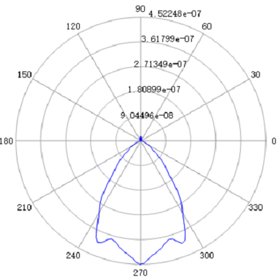
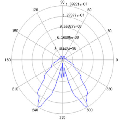
Example
# define phi in dashboard
phi = linspace(0, 360, 180);
# 3D simulation of 1D farfield
# define the projection plane
x = -sind(phi);
y = cosd(phi);
z = 0;
# calculate far field
myname = "far field from a closed box::xp";
nearfield = farfieldeqlprepareneardata(myname);
[Ex_xp, Ey_xp, Ez_xp] = farfieldeql(x, y, z,nearfield);
# show the far field
figure;
polar(phi*pi/180, abs(Ex_xp),'b');
figure;
polar(phi*pi/180, abs(Ey_xp),'b');
figure;
polar(phi*pi/180, abs(Ez_xp),'b');
Result:
abs(Ex_xp):

abs(Ey_xp):
abs(Ez_xp):
See also
farfieldeqlprepareneardata, farfieldeql2d
farfieldeql2d #
Description
farfieldeql2d projects any surface fields from the pre-defined monitors to a series of points defined by vector lists. The X/Y/Z coordinates of each evaluatation point are generated from the vector lists as the 2D/3D grid coordinates. This command returns three electric field components Exff,Eyff,Ezff in Cartesian coordinate system. This function can be used both in 2D and 3D simulation.
Calculate the far field projection on 2D projection surface.
Used in FDTD.
Syntax
| Code | Function |
|---|---|
[Ex, Ey, Ez] = farfieldeql2d(z, x, 0, nearfield, index_n2f); |
Returns the far field projection including three electric field components Exff,Eyff,Ezff in Cartesian coordinate system, which can be used in 2D simulation. The size of each component is determined by the length of z, x vector. |
[Ex, Ey, Ez] = farfieldeql2d(x, y, z, nearfield, index_n2f); |
Returns the far field projection including three electric field components Exff,Eyff,Ezff in Cartesian coordinate system, which can be used in 3D simulation. The size of each component is determined by the length of x, y, z vector. |
The meanings of the parameters in the above tabulation are illustrated as following:
| name | type | default | description |
|---|---|---|---|
| x | vector | - | The x coordinates of the grid points where far field is calculated. Column vector is recommended. The length of X is M or 1. |
| y | vector | - | The y coordinates of the grid points where far field is calculated. Column vector is recommended. The length of Y is N or 1. |
| z | vector | - | The z coordinates of the grid points where far field is calculated. Column vector is recommended. The length of Z is P or 1. |
| nearfield | struct | - | The near field data prepared for far field projection from the farfieldeqlprepareneardata function. |
| index_n2f | num | 1 (optional) | The background refractive index of the transmission process from near-field to far-field. |
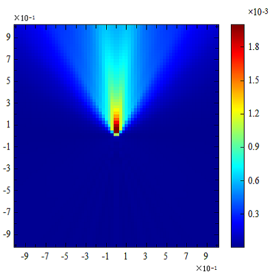
Example
# 2D simulation of 2D farfield
# define the projection plane
z = linspace(-1, 1, 72);
x = linspace(-1, 1, 70);
y = 0;

# calculate farfield
myname = "far field from a closed box::zp";
nearfield = farfieldeqlprepareneardata(myname);
[Ez_xp, Ex_xp, Ey_xp] = farfieldeql2d(z, x, 0, nearfield);

# show the far field
figure;
image(x, z, abs(Ex_xp));
figure;
image(x, z, abs(Ey_xp));
figure;
image(x, z, abs(Ez_xp));
Result:
Ex_xp:
Ey_xp:
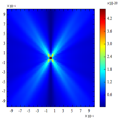
Ez_xp:
Reference
C. A. Balanis, Antenna Theory and Design, 4th Edition. John Wiley & Sons , 2016.
See also
farfieldeqlprepareneardata, farfieldeql
far-field angular spectrum method #
The far-field angular spectrum method functions involve farfieldas and farfieldpolar, which can quickly obtain the far field projection in Cartesian and spherical coordinate systems.
farfieldas #
Description
Returns far fields decomposed into plane wave spectrum (or Fourier series). In a 3D simulation, the far field is projected to a 1-meter hemisphere, while in a 2D simulation, it is projected to a 1-meter semicircular ring.
Syntax
| Code | Function |
|---|---|
[Exfm, Eyfm, Ezfm] = farfieldas(myname, lambda_i, index, k_num1, k_num2); |
Projecting the given FDFP monitor to the far field, where index specifies the refractive index at the location of the FDFP monitor. Returns the far field projection including three electric field components Exfm,Eyfm,Ezfm in Cartesian coordinate system, which can be used in 3D simulation. This returns an N×M matrix if 1 wavelength point is projected, or a N×M×P matrix if more than 1 wavelength point is projected, where N and M correspond to the resolution of the projection (k_num1, and k_num2), and P corresponds to the number of frequency points projected. |
[Exfm, Eyfm, Ezfm] = farfieldas(myname, lambda_i, index, k_num1 ); |
Projecting the given FDFP monitor to the far field, where index specifies the refractive index at the location of the FDFP monitor. Returns the far field projection including three electric field components Exfm,Eyfm,Ezfm in Cartesian coordinate system, which can be used in 2D simulation. The result is an N×M matrix where the first dimension is the resolution of the far field projection, and the second dimension is the number of wavelength points projected. |
The meanings of the parameters in the above tabulation are illustrated as following:
| name | type | default | description |
|---|---|---|---|
| myname | string | -- | the name of the FDFP monitor |
| lambda_i | vector | 1 | the serial number of wavelength points |
| index | number | 1 | the index at the FDFP monitor center |
| k_num1 | number | 200(3D), 1000(2D) | the number of samples of kx |
| k_num2 | number | 200(3D) | the number of samples of ky |
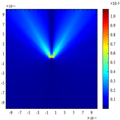
Example
This example demonstrates how to calculate the far field of a 3D monitor. The electric field intensity ∣E∣2 is used to represent far field results.
# 3D simulation
# 1m far-field hemisphere
k_num1 = 200;
k_num2 = 200;
ux = linspace(-1,1,k_num1);
uy = linspace(-1,1,k_num2);

myname = "FDTD::field";
[Exfm, Eyfm, Ezfm] = farfieldas(myname, 1, 1, k_num1, k_num2);
E2 = abs(Exfm).^2 + abs(Eyfm).^2 + abs(Ezfm).^2;
image(ux, uy, E2);
∣E∣2:
See also
farfieldeql, farfieldeql2d
farfieldpolar #
Description
Returns far fields in a spherical coordinate system that is decomposed into plane wave spectrum (or Fourier series) in 2D or 3D simulation. For 3D simulation, it returns Er,Eθ,Eϕ. For 2D simulation, it returns Er,Eθ,Ez.
Syntax
| Code | Function |
|---|---|
[Er, Eth, Ephi] = farfieldpolar(myname, lambda_i, index, k_num1, k_num2); |
Projecting the given FDFP monitor to the far field, where index specifies the refractive index at the location of the FDFP monitor. Returns the far field projection including three electric field components Er,Eθ,Eϕ in spherical coordinate system, which can be used in 3D simulation. This returns an N×M matrix if 1 wavelength point is projected, or a N×M×P matrix if more than 1 wavelength point is projected, where N and M correspond to the resolution of the projection (k_num1, and k_num2), and P corresponds to the number of frequency points projected. |
[Er, Eth, Ez] = farfieldpolar(myname, lambda_i, index, k_num1); |
Projecting the given FDFP monitor to the far field, where index specifies the refractive index at the location of the FDFP monitor. Returns the far field projection including three electric field components Er,Eθ,Ez in spherical coordinate system, which can be used in 2D simulation. The result is an N×M matrix where the first dimension is the resolution of the far field projection, and the second dimension is the number of wavelength points projected. |
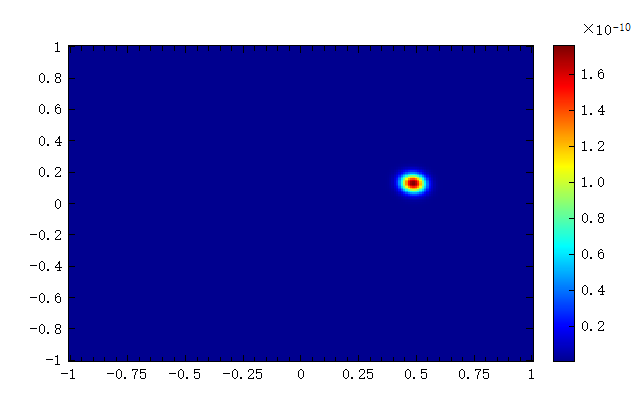
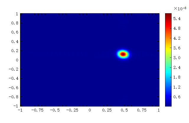
Example
This example demonstrates how to calculate the far field of a specified monitor.
# 3D simulation
# 1m far-field hemisphere
k_num1 = 200;
k_num2 = 200;
ux = linspace(-1, 1, k_num1);
uy = linspace(-1, 1, k_num2);

myname = "FDTD::field";
[Er, Eth, Ephi] = farfieldpolar(myname, 1, 1, k_num1, k_num2);
figure;
image(ux, uy, abs(Er));
figure;
image(ux, uy, abs(Eth));
figure;
image(ux, uy, abs(Ephi));
abs(Er):

abs(Eth):

abs(Ephi):
See also
farfieldas
farfield2dintegrate #
Description
Calculate the integration of far-field projection over a certain range of theta in 2D simulation.
Syntax
| Code | Function |
|---|---|
E2_integrate = farfield2dintegrate(E2, theta, theta0, halfangle) |
Returns the integration of far-field projection over a certain range of theta in 2D simulation. |
The meanings of the parameters in the above tabulation are illustrated as following:
| name | type | default | description |
|---|---|---|---|
| E2 | matrix | -- | The electric field intensity from farfieldas in 2D simulation. |
| theta | vector | -- | The projection angle of the far-field semicircular ring. |
| theta0 | num | 0 | Center angle of the integration range. Theta0 should be between -90 to 90 degrees. |
| halfangle | num | 90 | Half angle width of the integration range. Halfangle should be between 0 to 90 degrees. |
Notice: While the angles are provided in degrees, the actual integration is executed in radians.
Example
k_num = 1000;
ut = linspace(-1, 1, k_num);
myname = "FDTD::field";
[Exfm, Eyfm, Ezfm] = farfieldas(myname, 1, 1, k_num);
E2 = abs(Exfm).^2 + abs(Eyfm).^2 + abs(Ezfm).^2;
theta=asind(ut);
E2_integrate = farfield2dintegrate(E2, theta, 0, 90)
Result:
E2_integrate = 2.29694839e-06
Reference
Allen Taflove, Computational Electromagnetics: The Finite-Difference Time-Domain Method. Boston: Artech House, 2005.
grating analysis #
The grating functions involve grating、 gratingvector、gratingpolar、gratingorder、gratingperiod、gratingu and gratingordercount, which can be conveniently used to calculate the far-field from a periodic grating structure.
If your structure is not periodic, see the far-field analysis.
grating #
Returns the fraction of transmitted power to each physical grating orders for a given simulation. Results are normalized such that the sum of all the orders is equal to 1. To convert these values into fractions of the source power, multiply by the transmittance of the monitor.
3D simulations: Data is returned in a N×M×P matrix where N, M are the number of grating orders, and P is the number of frequency points.
2D simulations: Data is returned in a N×P matrix where N is the number of grating orders, and P is the number of frequency points.
Syntax
| Code | Function |
|---|---|
G=grating(myname,K,f_ind,index); |
Returns the strength of all physical grating orders from FDFP monitor named "myname". |
The meanings of the parameters in the above tabulation are illustrated as following:
| name | type | default | description |
|---|---|---|---|
| mname | string | - | The name of the FDFP monitor |
| K | vector | [0,0,0] | The Bloch vector of the injected source |
| f_ind | vector | The index of the frequency point with the highest number of grating orders | The index of the desired frequency point. This can be a single number or a vector. |
| index | number | The background index | The index of the material to use for the projection |
The following table summarizes how to interpret the coordinate vector properties for various monitor orientations.
| Monitor orientation | Monitor surface normal | first dimension | 2nd dimension |
|---|---|---|---|
| XY plane | Z | x axis | y axis |
| XZ plane | Y | x axis | z axis |
| YZ plane | X | y axis | z axis |
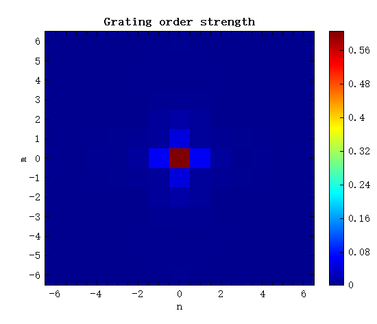
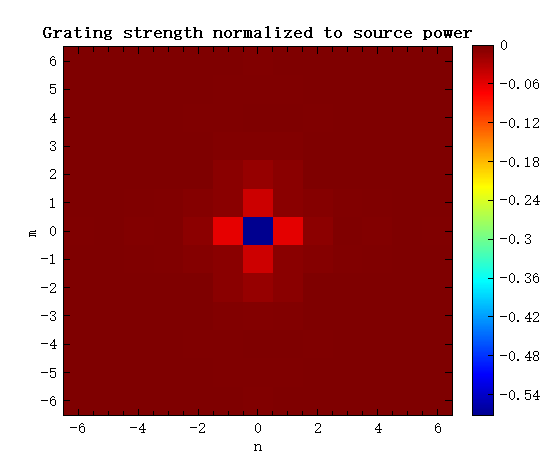
Example
mname = "FDTD::trans";
K = [0,0,0];
f_index = 1;
[n,m] = gratingorder(mname,K,f_index);# grating order numbers
[~,u1,u2] = gratingu(mname,K,f_index);# grating unit vectors
G = grating(mname,K,f_index);         # power to each order (fraction of transmitted power)
T = real(getdata(mname,"T","T"));     # total power transmitted through monitor (fraction of source power)

figure;
image(n,m,G');
xlabel("n");
ylabel("m");
title("Grating order strength");

figure;
image(n,m,(G.*T(f_index))');
xlabel("n");
ylabel("m");
title("Grating strength normalized to source power");
Result:
See also
gratingvector, gratingpolar, gratingorder, gratingu, gratingperiod, gratingordercount
gratingvector #
Returns the relative strength of all physical grating orders where vector field information is returned in Cartesian coordinates. This is useful when studying the polarization effects. The data is normalized such that the sum of ∣Ex∣2+∣Ey∣2+∣Ez∣2 over all grating orders equals 1.
Syntax
| Code | Function |
|---|---|
[Ex,Ey,Ez]=gratingvector(myname,K,f_ind,index); |
Returns the strength of all physical grating orders from FDFP monitor named "myname". Output is in Cartesian coordinates. |
The meanings of the parameters in the above tabulation are same as grating function.
Example
mname = "FDTD::trans";
K = [0,0,0];
f_index = 1;
[Ex,Ey,Ez] = gratingvector(mname,K,f_index)
G = grating(mname,K,f_index)
abs(Ex).^2+abs(Ey).^2+abs(Ez).^2 # gratingvector gives the same result as the grating function
                                 # when we calculate |Ex|^2+|Ey|^2+ |Ez|^2.
Result:
Ex =
   0.0472510232 +0.0842199759i
   0.0517839815 -  0.57081118i
    0.261147775 - 0.235296591i
   0.0517839815 -  0.57081118i
   0.0472510232 +0.0842199759i

Ey =
              0 +           0i
              0 +           0i
              0 +           0i
              0 +           0i
              0 +           0i

Ez =
  -0.0814970775 -    0.144839i
  -0.0249681964 + 0.268593577i
-5.29711237e-17 -3.97206664e-17i
   0.0249681964 - 0.268593577i
   0.0814970775 +    0.144839i
G =
  0.0369457731
   0.401272904
   0.123562646
   0.401272904
  0.0369457731
val =
  0.0369457731
   0.401272904
   0.123562646
   0.401272904
  0.0369457731
See also
grating, gratingpolar, gratingorder, gratingu, gratingperiod, gratingordercount
gratingpolar #
Returns the relative strength of all physical grating orders where vector field information is returned in spherical coordinates. This is useful when studying the polarization effects. The data is normalized such that the sum of ∣Er∣2+∣Eθ∣2+∣Eϕ∣2 over all grating orders equals 1.
Syntax
| Code | Function |
|---|---|
[Er,Et,Ep]=gratingpolar(myname,K,f_ind,index); |
Returns the strength of all physical grating orders from FDFP monitor named "myname". Output is in spherical coordinates. |
The meanings of the parameters in the above tabulation are same as grating function.
Example
mname = "FDTD::trans";
K = [0,0,0];
f_index = 1;
[Er,Et,Ep] = gratingpolar(mname,K,f_index)
G = grating(mname,K,f_index)
abs(Er).^2+abs(Et).^2+abs(Ep).^2 # gratingpolar gives the same result as the grating function
                                 # when we calculate |Er|^2+|Et|^2+ |Ep|^2.
Result:
Er =
  -0.0419574402 +0.0158414336i
    0.292753618 + 0.076306164i
5.80038415e-18 +1.77830992e-17i
   -0.292753618 - 0.076306164i
   0.0419574402 -0.0158414336i

Et =
 -0.0248656245 +0.00813802798i
    -0.24094981 -0.0631413769i
    0.817516808 - 0.138320454i
    -0.24094981 -0.0631413769i
 -0.0248656245 +0.00813802798i

Ep =
              0 +           0i
              0 +           0i
              0 +           0i
              0 +           0i
              0 +           0i
G =
 0.00269590458
   0.153570956
   0.687466279
   0.153570956
 0.00269590458
val =
 0.00269590458
   0.153570956
   0.687466279
   0.153570956
 0.00269590458
See also
grating, gratingvector, gratingorder, gratingu, gratingperiod, gratingordercount
gratingorder #
Description
Returns the vector of the grating order numbers(i.e. zero order, first order). This function can be used both in 2D and 3D simulation. The "m" can only be returned in 3D simulation.
Used in FDTD.
Syntax
| Code | Function |
|---|---|
n=gratingorder(myname,K,f_ind,index); |
Returns the vector of the grating order numbers for the first dimension. The "n" is returned in a N×P matrix where N is the number of grating orders, and P is the number of frequency points. |
[n,m]=gratingorder(myname,K,f_ind,index); |
Returns the vector of the grating order numbers for two dimensions. The "m" is returned in a M×P matrix where M is the number of grating orders, and P is the number of frequency points. |
The meanings of the parameters in the above tabulation are same as grating function.
Example
# 3D simulation
myname="FDTD::trans";   # FDFP monitor name
K=[0,0,0];  #Bloch vector of the injected source
f_ind=1;    #the index of the desired frequency point
index=3.5;  #the index of the material to use for the projection
[n,m]=gratingorder(myname,K,f_ind,index)
Result:
n =
            -3
            -2
            -1
             0
             1
             2
             3

m =
            -3
            -2
            -1
             0
             1
             2
             3
See also
grating, gratingvector, gratingpolar, gratingu, gratingperiod, gratingordercount
gratingu #
Description
Returns the angle vector of each grating order, in degrees, for 2D simulations. Or returns the grating order direction unit vectors(u1 and u2) for 3D simulation.
Syntax
| Code | Function |
|---|---|
angle=gratingu(myname,K,f_ind,index); |
Returns the angle vector corresponding to the grating order numbers for the first dimension. The "angle" is returned in a N×P matrix where N is the number of grating orders, and P is the number of frequency points. |
[~,u1]=gratingu(myname,K,f_ind,index); |
Returns the direction unit vectors corresponding to the grating order for the first dimension. The "u1" is returned in a N×P matrix where N is the number of grating orders, and P is the number of frequency points. |
[~,~,u2]=gratingu(myname,K,f_ind,index); |
Returns the direction unit vectors corresponding to the grating order for the 2nd dimension. The "u2" is returned in a M×P matrix where M is the number of grating orders, and P is the number of frequency points. |
The meanings of the parameters in the above tabulation are same as grating function.
Example
myname="FDTD::trans";   # FDFP monitor name
K=[0,0,0];  #Bloch vector of the injected source
f_ind=3;    #the index of the desired frequency point
index=3.5;  #the index of the material to use for the projection
angle=gratingu(myname,K,f_ind,index)
[~,u1]=gratingu(myname,K,f_ind,index)
[~,~,u2]=gratingu(myname,K,f_ind,index)
Result
angle =
   -58.9972809
   -25.3769335
             0
    25.3769335
    58.9972809

u1 =
  -0.857142857
  -0.428571429
             0
   0.428571429
   0.857142857

u2 =
  -0.857142857
  -0.428571429
             0
   0.428571429
   0.857142857
See also
grating, gratingvector, gratingpolar, gratingorder, gratingperiod, gratingordercount
gratingperiod #
Description
Returns the grating period (i.e. the simulation span) used in the grating calculations.
Syntax
| Code | Function |
|---|---|
d1=gratingperiod(myname); |
Returns the period for the first dimension(2D and 3D). |
[d1,d2]=gratingperiod(myname); |
Returns the period for the 1st and 2nd dimension(3D only). |
The meanings of the parameter in the above tabulation is illustrated as following:
| name | type | default | description |
|---|---|---|---|
| mname | string | - | The name of the FDFP monitor |
Example
[d1,d2]=gratingperiod(myname)
Result
d1 =
         2e-07

d2 =
         2e-07
See also
grating, gratingvector, gratingpolar, gratingorder, gratingu, gratingordercount
gratingordercount #
Description
Returns the total number of supported grating numbers.
Syntax
| Code | Function |
|---|---|
Count=gratingordercount(myname,K,f_ind,index) |
Returns the total number of supported grating orders. |
The meanings of the parameters in the above tabulation are same as grating function.
Example
myname="FDTD::trans";   # FDFP monitor name
K=[0,0,0];  #Bloch vector of the injected source
f_ind=[1,2,3];    #the index of the desired frequency point
index=3.5;  #the index of the material to use for the projection
Count=gratingordercount(myname,K,f_ind,index)
Result
Count =
           145
            37
            21
See also
grating, gratingvector, gratingpolar, gratingorder, gratingu, gratingperiod
Inverse Design #
topoparamstoindex #
Description
topoparamstoindex is a dedicated script function for topology optimization in inverse design, and it is exclusively used in the topology optimization workflow of inverse design. The core function of this function is to map the topology optimization parameters of the device structure to the corresponding permittivity distribution.
Syntax
| Code | Function |
|---|---|
eps = topoparamstoindex(params, rho); |
params is a structure that controls the filter parameters. rho is the original structural parameter matrix in topology optimization (normalized to the range [0,1]). eps is the permittivity distribution output by topology optimization (with the same matrix dimension as rho). |
params Structure Parameter Description
| Name | Unit | Default | Description |
|---|---|---|---|
beta |
1 | The steepness of the filter optimization. The larger the value, the steeper the transition of the topology parameters, and the clearer the gradient characteristics of the objective function. | |
dx/dy/dz |
m | The width setting of the filter. Currently, only 2D topology optimization is supported, and dz needs to be set to 0. |
|
eps_levels |
The permittivity levels, corresponding to the permittivity when the topology parameter rho=0 and rho=1 respectively. The second value needs to be larger than the first one. |
||
eta |
0.5 | The binarization threshold of the filter. When the value is less than 0.5, the optimization tends to the permittivity corresponding to rho=0; when the value is greater than 0.5, it tends to the permittivity corresponding to rho=1. |
|
filter_radius |
m | 2e-7 | The filter radius, which determines the minimum length of the feature size and smoothes the structural optimization. |
Example
clear;
clc;

params = struct(beta=1;dx=2e-8;dy=2e-8;dz=0;eps_levels=[2.0736,7.84];eta=0.5;filter_radius=5e-7); # Configure filter parameters
rho = rand(100, 100); # Generate random topology optimization parameters
eps = topoparamstoindex(params, rho);
See also
topoparamstogradient
topoparamstogradient #
Description
topoparamstogradient is used in the inverse design workflow to calculate the gradient field of the objective function with respect to the topology optimization parameters. It is synergistic with topoparamstoindex.
Syntax
| Code | Function |
|---|---|
dF_drho = topoparamstogradient(params, rho, dF_dEps); |
The parameters params and rho are consistent with the requirements of topoparamstoindex. dF_dEps is the gradient field of the objective function with respect to the permittivity distribution. dF_drho is the output gradient field of the objective function with respect to the original topology parameters. |
See also
topoparamstoindex
topoparamstominfeaturesizeindicator #
Description
In topology optimization, topoparamstominfeaturesizeindicator is a low-level core function that computes the minimum feature size constraint metric for the current design. Together with topoparamstominfeaturegradient, it forms the automated implementation mechanism for minimum feature size constraints, ensuring a balance between manufacturability (i.e., satisfying minimum line width and spacing requirements) and performance.
Syntax
| Code | Function |
|---|---|
indicator = topoparamstominfeaturesizeindicator(params, rho); |
params is a structure controlling the feature size constraint and filtering parameters. rho is the original design variable matrix. indicator is a scalar representing the degree of violation of the constraint for the current design. |
params Structure Parameter Description
| Name | Unit | Default | Description |
|---|---|---|---|
filter_radius |
m | 2e-7 | Filter radius, defining the precision of the size constraint. |
beta |
12 | Steepness of the projection filter; larger values lead to sharper transitions between materials. | |
eta |
0.5 | Binarization threshold; values are in the range [0,1]. Values <0.5 bias the design toward the lower permittivity material, >0.5 toward the higher permittivity material. | |
dx / dy / dz |
m | Grid spacing in the design region. For 2D topology optimization, dz must be set to 0. |
Example
clearall;

params=struct;
params.dx=2e-8;
params.dy=2e-8;
params.dz=0;
params.filter_radius=500e-9;
params.eta=0.5;
params.beta=12;
params.eta_e=0.75;
params.eta_d=0.25;

topo_rho=zeros(151,91);

topo_rho(30:40,:)=1;
topo_rho(20:30,20:30)=0.75;
topo_rho(50:75,50:75)=1;
topo_rho(80:85,80:85)=0.5;

# compute the indicator that violate the mini-feature
violation = topoparamstominfeaturesizeindicator(params,topo_rho)
See also
topoparamstominfeaturegradient
topoparamstominfeaturegradient #
Description
topoparamstominfeaturegradient is a low-level function in topology optimization used to compute the gradient of the minimum feature size constraint. It works in conjunction with topoparamstominfeaturesizeindicator to provide gradient‑based optimizers with sensitivity information, guiding the design toward satisfying manufacturability constraints while optimizing performance.
Syntax
| Code | Function |
|---|---|
grad = topoparamstominfeaturegradient(params, rho); |
params is a structure controlling the feature size constraint and filtering parameters (same as in topoparamstominfeaturesizeindicator). rho is the design variable matrix. grad is a matrix of the same size as rho containing the gradient of the constraint indicator with respect to each design variable. |
Example
clearall;

params=struct;
params.dx=2e-8;
params.dy=2e-8;
params.dz=0;
params.filter_radius=500e-9;
params.eta=0.5;
params.beta=12;
params.eps_levels=[2.0736,7.84];
params.eta_e=0.9;
params.eta_d=0.1;

topo_rho=zeros(151,91);
topo_rho(:,30:60)=1;
topo_rho(35:55,35:55)=0;
topo_rho(60:80,60:80)=1;

# compute the indicator that violates the mini-feature
violation = topoparamstominfeaturesizeindicator(params, topo_rho)

dI_drho = topoparamstominfeaturegradient(params, topo_rho);

figure;
image(dI_drho)
See also
topoparamstominfeaturesizeindicator
peaks #
Description
Generates a topographic map.
Used in FDTD and FDE.
Syntax
| Code | Function |
|---|---|
peaks(num); |
Returns a num * num result matrix according to the designated function. |
peaks(num_1, num_2); |
Returns a num_1 * num_2 result matrix according to the designated function. |
Example
maps = peaks(200,300);

figure;
image(maps);
title('maps');
Result:

focusingfield #
Description
Returns the focusing field including E(Ex,Ey,Ez), H(Hx,Hy,Hz) in the form of struct.
Used in FDTD and FDE.
Syntax
| Code | Function |
|---|---|
[E, H] = focusingfield(lambda, NA, k_num, index, distance); |
Returns the focusing field according to the input parameters. |
[E, H] = focusingfield(lambda, NA, k_num, index); |
Returns the focusing field according to the input parameters. In this case, distance is 0. |
[E, H] = focusingfield(lambda, NA, k_num); |
Returns the focusing field according to the input parameters. In this case, distance and index are 0 and 1 respectively. |
[E, H] = focusingfield(lambda, NA); |
Returns the focusing field according to the input parameters. In this case, distance, index, k_num are 0, 1 and 200 respectively. |
The meanings of the parameters in the above tabulation are illustrated as following:
| name | type | default | description |
|---|---|---|---|
| lambda | number | -- | wavelength(unit: m) |
| NA | number | -- | numerical aperture(unit: m) |
| k_num | number | 200 | the number of samples in k space |
| index | number | 1 | refractive index |
| distance | number | 0 | distance(unit: m) |
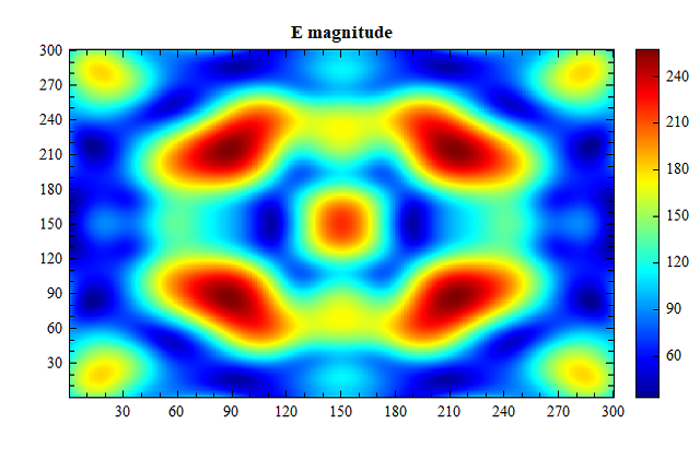
Example
[E, H] = focusingfield(1e-6, 2, 300, 1, 1);

E_mag = sqrt(abs(E.Ex).^2 + abs(E.Ey).^2 + abs(E.Ez).^2);

figure;
image(E_mag);
title('E magnitude');
Result:
See also
peaks
chromaticity #
The chromaticity functions involve chromatchfun, chromatch, chromatchxy, chromatchuv, lightsource, and chromaspacexy. Given the spectrum, the location in color space can be computed through the above functions. For instance, the spectrum under the test is shown below:
# create a dummy spectrum
lambda=linspace(380,700,1000); # unit: nm
spectrum = exp(-(lambda-550).^2./(30).^2);

# show spectrum
figure;
plot(lambda, spectrum);
xlabel('lambda (nm)');
ylabel('spectrum');
title('spectrum');
spectrum:
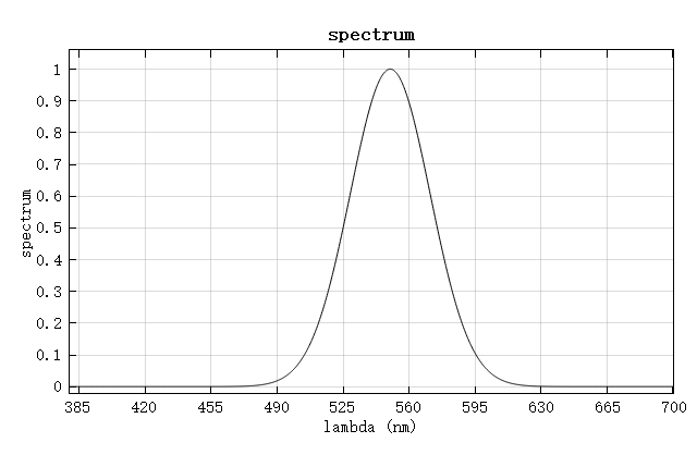
This spectrum is frequently used in the example part of chromaticity functions introduction.
chromatchfun #
Description
Returns the set xˉ, yˉ, zˉ of color matching functions of chromaticity system CIE 1931 or CIE 1964 in designated wavelength band (unit: nm), the result is dimensionless.
Used in FDTD and FDE.
Syntax
| Code | Function |
|---|---|
D = chromatchfun('chromaticity_system'); |
Gets the set of designated color matching functions in default wavelength band. The parameter 'chromaticity_system' can be 'CIE 1931' or 'CIE 1964'. The first row of the result D is the wavelength (unit: nm), the second, third and fourth rows of the result D are xˉ, yˉ, zˉ respectively. |
D = chromatchfun('chromaticity_system', lambda); |
Gets the set of designated color matching functions in wavelength band designated by wavelength parameter lambda. The parameter 'chromaticity_system' can be 'CIE 1931' or 'CIE 1964'. The first row of the result D is the wavelength (unit: nm), the second, third and fourth rows of the result D are xˉ, yˉ, zˉ respectively. |
Example
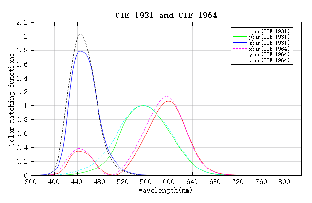
This example shows how to get the list of available color matching functions and plot them.
D1 = chromatchfun('CIE 1931'); # CIE 1931
D2 = chromatchfun('CIE 1964'); # CIE 1964

plot(D1(1, :), D1(2, :), 'r');
holdon;
plot(D1(1, :), D1(3, :), 'g');
holdon;
plot(D1(1, :), D1(4,: ), 'b');
holdon;
plot(D2(1, :), D2(2, :), 'm--');
holdon;
plot(D2(1, :), D2(3, :), 'c--');
holdon;
plot(D2(1, :), D2(4, :), 'k--');
legend('xbar(CIE 1931)', 'ybar(CIE 1931)', 'zbar(CIE 1931)', 'xbar(CIE 1964)', 'ybar(CIE 1964)', 'zbar(CIE 1964)');
xlabel('wavelength(nm)');
ylabel('Color matching functions');
title('CIE 1931 and CIE 1964');
Result:
See also
chromatch
chromatch #
Description
Returns the X, Y and Z tristimulus values calculated for a given spectral power distribution (power per unit wavelength per unit area) using the designated color matching functions of the chromaticity system( CIE 1931 or CIE 1964 ). The color matching function assumes that the wavelength of the spectral power distribution is in nanometers, W/(m2⋅nm).
Used in FDTD and FDE.
The expressions for the X, Y, and Z values are calculated as follows:
X=∫I(λ)xˉ(λ)dλ
Y=∫I(λ)yˉ(λ)dλ
Z=∫I(λ)zˉ(λ)dλ
where I(λ) is the spectral power distribution and xˉ,yˉ,zˉ are the color matching functions.
Syntax
| Code | Function |
|---|---|
[X,Y,Z] = chromatch(spectrum, lambda); |
Returns the X, Y, and Z tristimulus values calculated for spectral power distribution (power per unit wavelength per unit area) given by spectrum using the color matching functions of chromaticity system CIE 1931 in wavelength band (unit: nm) lambda. |
[X,Y,Z] = chromatch(spectrum, lambda, 'chromaticity_system'); |
Returns the X, Y and Z tristimulus values calculated for spectral power distribution (power per unit wavelength per unit area) given by spectrum using the designated color matching functions of chromaticity system 'chromaticity_system' in wavelength band (unit: nm) lambda. |
Example
# create a dummy spectrum
lambda = linspace(380, 700, 500);             # unit: nm
spectrum = exp(-(lambda-550).^2 ./ (30).^2);  # spectral power distribution


[X1, Y1, Z1] = chromatch(spectrum, lambda);
[X2, Y2, Z2] = chromatch(spectrum, lambda, 'CIE 1931');
[X3, Y3, Z3] = chromatch(spectrum, lambda, 'CIE 1964');
See also
chromatchfun
chromatchxy #
Description
Returns the x and y chromaticity values according to the input X, Y, and Z tristimulus values which are calculated by chromatch function. The chromatchxy function assumes that the wavelength unit of the spectral power distribution is nanometer, such as W/(m2⋅nm).
Used in FDTD and FDE.
x and y values are dimensionless and can be calculated as follows:
x=X+Y+ZX,y=X+Y+ZY
Syntax
| Code | Function |
|---|---|
[x, y] = chromatchxy(X, Y, Z); |
Returns the x and y chromaticity values according to the input X, Y, Z, which are calculated by chromatch function. |
Example
# create a dummy spectrum
lambda = linspace(380, 700, 500);             # unit: nm
spectrum = exp(-(lambda-550).^2 ./ (30).^2);  # spectral power distribution

[X1, Y1, Z1] = chromatch(spectrum, lambda);
[X2, Y2, Z2] = chromatch(spectrum, lambda, 'CIE 1931');
[X3, Y3, Z3] = chromatch(spectrum, lambda, 'CIE 1964');

[x2, y2] = chromatchxy(X2, Y2, Z2);
[x3, y3] = chromatchxy(X3, Y3, Z3);
See also
chromatchxy
chromatchuv #
Description
Returns the u′ and v′ chromaticity values according to the input X, Y and Z tristimulus values which are calculated by chromatch function. The chromatchuv function assumes that the wavelength unit of the spectral power distribution is nanometer, such as W/(m2⋅nm).
Used in FDTD and FDE.
u′ and v′ values are dimensionless and can be calculated as follows:
u′=X+15Y+3Z4X,v′=X+15Y+3Z9Y
Syntax
| Code | Function |
|---|---|
[u, v] = chromatchxy(X, Y, Z); |
Returns the u and v chromaticity values according to the input X, Y, Z, which are calculated by chromatch function. |
Example
# create a dummy spectrum
lambda = linspace(380, 700, 500);             # unit: nm
spectrum = exp(-(lambda-550).^2 ./ (30).^2);  # spectral power distribution

[X1, Y1, Z1] = chromatch(spectrum, lambda);
[X2, Y2, Z2] = chromatch(spectrum, lambda, 'CIE 1931');
[X3, Y3, Z3] = chromatch(spectrum, lambda, 'CIE 1964');

[u2, v2] = chromatchuv(X2, Y2, Z2);
[u3, v3] = chromatchuv(X3, Y3, Z3);
See also
chrmatchuv
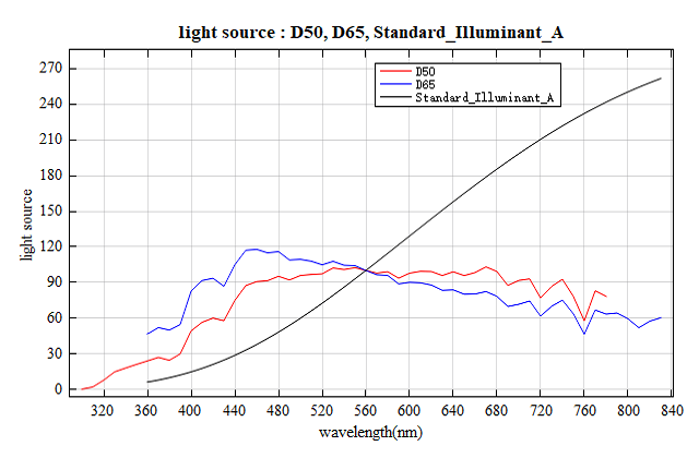
lightsource #
Description
Returns the desired set of light source from the available lists of D50, D65, or Standard Illuminant A.
Used in FDTD and FDE.
Syntax
| Code | Function |
|---|---|
S = lightsource('function'); |
Gets the desired set of light source from the list of available ones. In this function, the number 1 represents "D50", the number 2 represents "D65", and the number 3 represents "Standard Illuminant A". The first row of result matrix S is the wavelength (unit: nm), the second row is the relative radiance spectrum of the light source. |
Example
This example shows how to get the list of available light sources and plot them.
# The first row is the wavelength,(360-830), unit: nm
# The second row is the relative radiance spectrum of the light source.

D50 = lightsource('D50'); # D50
D65 = lightsource('D65'); # D65
Standard_Illuminant_A = lightsource('Standard Illuminant A'); # Standard Illuminant A

# plot
figure;
plot(D50(1, :),D50(2, :), 'r');
holdon;
plot(D65(1, :),D65(2, :), 'b');
holdon;
plot(Standard_Illuminant_A(1, :), Standard_Illuminant_A(2, :), 'k');
legend('D50', 'D65', 'Standard_Illuminant_A');
xlabel('wavelength(nm)');
ylabel('light source');
legend('D50', 'D65', 'Standard_Illuminant_A');
title('light source : D50, D65, Standard_Illuminant_A');
Result:
See also
chromaspacexy
chromaspacexy #
Description
Returns the x and y coordinates in the color space calculated using the given spectral power distribution (reflective cases), the light source, and color matching functions.
Used in FDTD and FDE.
The spectral power distribution is:
P(λ)=I(λ)R(λ)
where I(λ) is the relative radiance spectrum of the light source, R(λ) is the spectral power distribution(the simulated reflectance spectrum). The tristimulus values X,Y and Z are computed through:
X=K1∫Lxˉ(λ)P(λ)dλ
Y=K1∫Lyˉ(λ)P(λ)dλ
Z=K1∫Lzˉ(λ)P(λ)dλ
Here, xˉ,yˉ and zˉ are the CIE standard observer functions. The integrals are computed over the visible range L. K is the normalized constant:
K=∫Lyˉ(λ)I(λ)dλ
The CIE chromaticity coordinate (x,y,z) can be obtained by normalization:
x=X+Y+ZX
y=X+Y+ZY
z=X+Y+ZZ=1−x−y
It is noteworthy that only two values of (x,y,z) are independent, because the intensity of the incident light source is normalized.
Syntax
| Code | Function |
|---|---|
[x,y] = chromaspacexy(spectrum,light,lambda); |
Returns the x and y coordinates in the color space according to the given spectral power distribution designated by spectrum, the light source designated by light, and color matching function of the chromaticity system CIE 1931. |
[x,y] = chromaspacexy(spectrum,light,lambda,'chromaticity_system'); |
Returns the x and y coordinates in the color space according to the given spectral power distribution designated by spectrum, the light source designated by light, and color matching function of chromaticity system designated by 'chromaticity_system'. The parameter 'chromaticity_system' can be 'CIE 1931' or 'CIE 1964'. |
Example
# create a dummy spectrum
lambda = linspace(380, 700, 500); # unit: nm
spectrum = exp(-(lambda-550).^2./(30).^2); # spectrum

# light source using D65
light_D65 = lightsource('D65');

# to gain the light source in desired wavelength points
light_source=interp(light_D65(2, :), light_D65(1, :), lambda);

light=[lambda; light_source];

[x, y] = chromaspacexy(spectrum, light, lambda, 'CIE 1931');
overlap #
In the FDE solver, users can calculate the overlap integral and power coupling between two modes through the Mode Workspace window and Overlap window. The same functionality can also be achieved using the bestoverlap function in scripts.
bestoverlap #
Description
Before using the bestoverlap function, the target mode for comparison (e.g., model_1) must first be added to the Mode Workspace. After re-solving for the modes, this function will calculate the index of the mode in the current mode list (e.g., model_2) that best matches the target mode stored in the Mode Workspace.
The overlap integral is calculated using the following formula:
overlap=∣∣∣∣∣∣Re[∫E1×H1∗dS(∫E1×H2∗dS)(∫E2×H1∗dS)]⋅Re(∫E2×H2∗dS)1∣∣∣∣∣∣
Syntax
| Code | Function |
|---|---|
mode_id = bestoverlap('mode_name'); |
Calculates the index of the mode that best matches the target mode mode_name. mode_name is the name of the target mode stored in the Mode Workspace, and mode_id is the index of the best matching mode in the current mode list. |
Example
In the case study Polarization Converter Using A Tapered Waveguide, model_3 is used as the target mode for matching. After re-solving for the modes, model_4 in the mode list is identified as the best matching mode.
mode_id = bestoverlap('model_3')
Result:
mode_id = 4
