This section introduces the functions providing various kinds of methods to visualize data.

Graphics

plot

Description
Plots a 2D line plot according to the designated data.
Used in FDTD and FDE.

Syntax

Code	Function
`plot(X, Y);`	Plots a 2D figure according to the data X, Y.
`plot(X, Y, 'line_type');`	Plots a 2D figure with specified line style, marker and color designated by 'line_type' according to the data X, Y.

There are the line styles, markers and colors that can be used:

(1) line styles:

Code	Line Style	Display
`'-'`	solid line style
`'--'`	dashed line style
`':'`	dotted line style
`'-.'`	dash-dot line style

(2) line markers:

Code	Marker	Display
`'+'`	plus marker
`'o'`	circle marker
`'*'`	star marker
`'.'`	dot marker
`'x'`	cross marker
`'s'`	square marker
`'d'`	diamond marker
`'^'`	upward triangle marker
`'v'`	downward triangle marker
`'<'`	leftward triangle marker
`'>'`	rightward triangle marker
`'p'`	pentagram marker
`'h'`	hexagram marker

(3) line colors:

Code	Color	Display
`'k'`	black
`'r'`	red
`'g'`	green
`'b'`	blue
`'c'`	cyan
`'m'`	magenta
`'y'`	yellow
`'w'`	white

Example
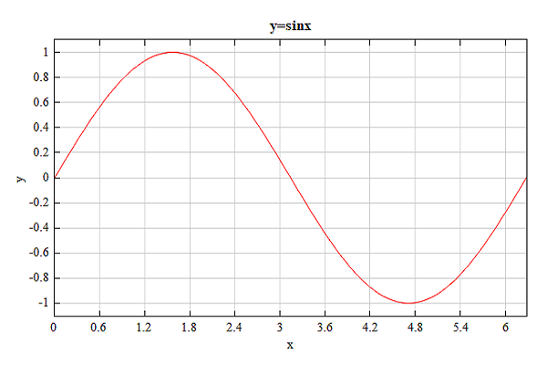
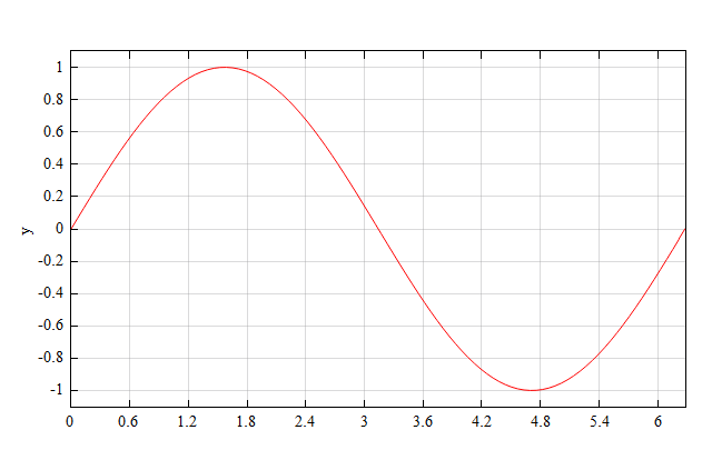
Plot the sin function.

# prepare data
pi = 3.1415926;
x = linspace(0, 2*pi, 100);
y = sin(x); 

# plot sine function
figure; 
plot(x, y, 'r'); 
title('y=sinx');  
xlabel('x'); 
ylabel('y');

Result:

See also
figure

plotyy

Description
Creates 2D line plots with two y-axes.
Used in FDTD and FDE.

Syntax

Code	Function
`plotyy(x1, y1, x2, y2);`	Plots y1 versus x1 with y-axis labeling on the left and plots y2 versus x2 with y-axis labeling on the right.
`plotyy(x1, y1, x2, y2, 'line_type_1', 'line_type_2');`	Plots y1 versus x1 with y-axis labeling on the left and plots y2 versus x2 with y-axis labeling on the right with designated line type.

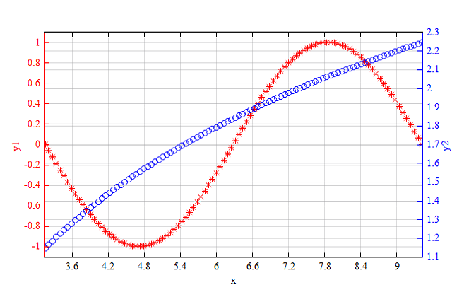
Example

x=linspace(pi, 3*pi);
y1 = sin(x);
y2 = log(x);

figure;
plotyy(x, y1, x, y2, '*r', 'ob');
xlabel('x');
ylabel('y1');
ylabel2('y2');

Result:

See also
plot

image

Description
Draws an image according to the designated data.
Used in FDTD and FDE.

Syntax

Code	Function
`image(z);`	Draws an image according to the designated data z.
`image(x, y, z);`	Draws an image according to the designated data z versus x, y.

Example
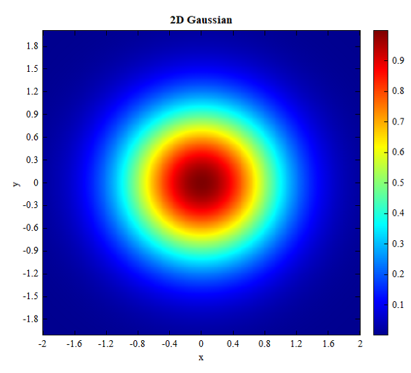
Show the 2D Gaussian distribution using image function.

# prepare data
x0 = linspace(-2, 2, 500);
y0 = linspace(-2, 2, 500);
[x,y] = meshgrid(x0, y0);
d = sqrt(x.^2 + y.^2);
E = exp(-(d).^2); # 2D Guassian distribution

# show image
figure;
image(x0, y0, E);
xlabel('x');
ylabel('y');
title('2D Gaussian');

Result:

See also
figure, plot

surf

Description
Draws a 3D spatial curved surface.
Used in FDTD and FDE.

Syntax

Code	Function
`surf(F);`	Draws a 3D spatial curved surface according to F data.
`surf(x, y, F);`	Draws a 3D spatial curved surface according to F versus x, y. The parameter x, y can be vectors or matrices.
`surf(x, y, Z, F);`	Draws a 3D spatial curved surface according to F versus x, y, z. The F data is manifested by color, and the parameters x, y, z are the coordinates data. The parameter x, y can be vectors or matrices but Z must be matrix with the same dimensions as F.

The following picture illustrates the surf function how to handle the input parameters:

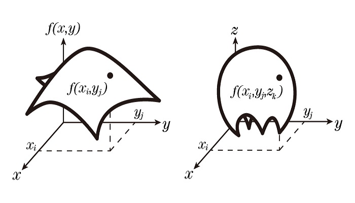
when using surf(x, y, F):
(1)If x, y are vectors, vector x has the length M, and y has the length N, and the surface data F has the size M * N.
(2)If x, y are matrices, then matrix x, y, F have the same size M * N.
when using surf(x, y, Z, F):
(1)If x, y are vectors, x has the length M, y has the length N, Z and F have the same size M * N.
(2)If x, y are matrices, then matrix x, y, Z, F have the same size M * N.

Example

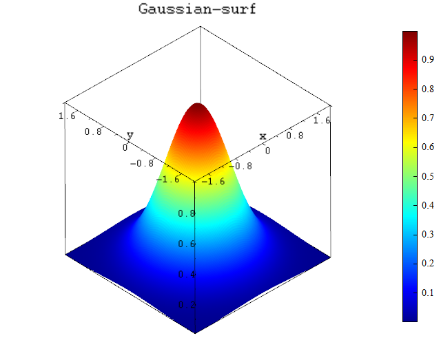
Example 1:
Draw the Gaussian distribution E as function of x, y using surf function.

# prepare data
x0 = linspace(-2, 2, 200);
y0 = linspace(-2, 2, 200);
[x,y] = meshgrid(x0, y0);
d = sqrt((x-0).^2 + (y-0).^2);
E = exp(-(d).^2); # 2D Guassian distribution

# show image
figure;
surf(x0,y0,E);
xlabel('x');
ylabel('y');
title('Gaussian-surf');

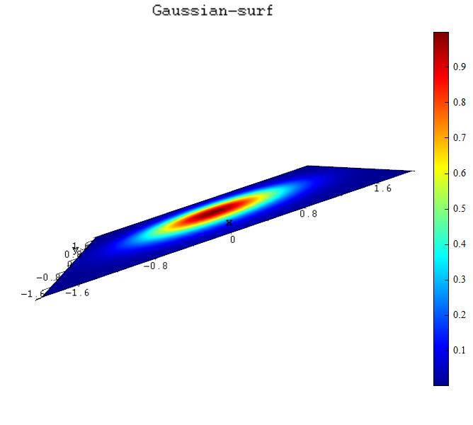
Example 2:
When input 4 parameters, and 3rd parameter defines the position in z-axis, and the 4th parameter determines the color of surface.
Continue running the following code after running code in example 1.

z = zeros(size(x)); # set z all to 0
figure;
surf(x, y, z, E);
xlabel('x');
ylabel('y');
title('Gaussian-surf');

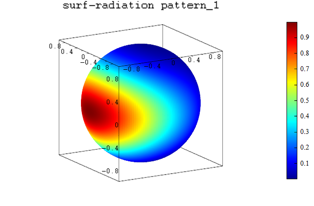
Example 3:

Generally, the surf function uses three inputs enough, but when drawing a radiation map, all 4 parameters needed.
Draw radiation map using surf function.

# prepare E data in Cartesian coordinate system
x0 = linspace(-2, 2, 200);
y0 = linspace(-2, 2, 200);
[x,y] = meshgrid(x0, y0);
d = sqrt((x-0).^2 + (y-0).^2);
E = exp(-(d).^2); # 2D Guassian distribution

# when in spherical coordinate system
E_size = size(E);
numv = E_size(1);
numt = E_size(2);

theta = linspace(0, pi, numv);   # theta [0, pi]
phi = linspace(0, 2*pi, numt);   # phi [0, 2*pi]
[T,U] = meshgrid(phi, theta);

# convert  spherical coordinate theta,phi,r to Cartesian coordiante x,y,z  
X = sin(U).*cos(T);
Y = sin(U).*sin(T);
Z = cos(U);

# surf draw
figure;
surf(X, Y, Z, abs(E));
title('surf-radiation pattern_1');


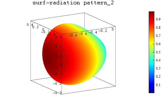
X = sin(U).*cos(T).*abs(E);
Y = sin(U).*sin(T).*abs(E);
Z = cos(U).*abs(E);


figure();
surf(X, Y, Z, abs(E));
title('surf-radiation pattern_2');

Result :

mesh

Description
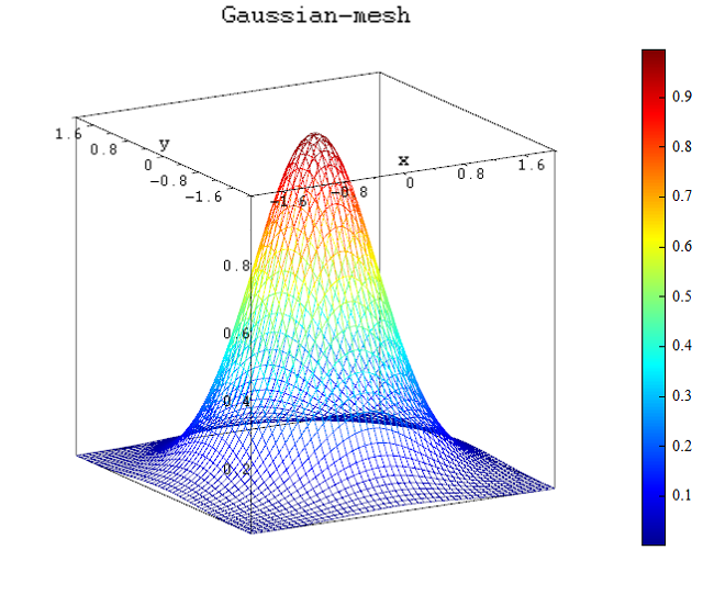
Draws a 3D wireframe mesh plot.
Used in FDTD and FDE.

Syntax

Code	Function
`mesh(F);`	Draws a 3D wireframe mesh plot according to F data.
`mesh(x, y, F);`	Draws a 3D wireframe mesh plot according to F data versus x, y. The parameter x, y can be vectors or matrices.

Example


x0 = linspace(-2, 2, 50);
y0 = linspace(-2, 2, 50);
[x,y] = meshgrid(x0, y0);
d = sqrt((x-0).^2 + (y-0).^2);
E = exp(-(d).^2); # 2D Guassian distribution

# show image
figure();
mesh(x0, y0, E);
xlabel('x');
ylabel('y');
title('Gaussian-mesh');

Result:

See also
surf

vectorplot

Description
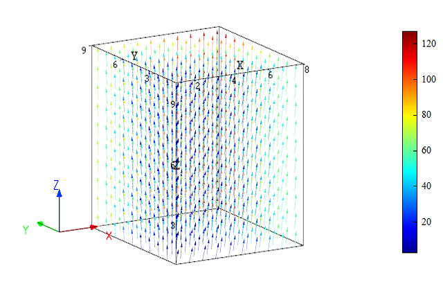
Creates a vector plot by axis and data (like E field).
Used in FDTD and FDE.

Syntax

Code	Function
`vectorplot(x, y, z, Ex, Ey, Ez)`	Creates a vector plot. The parameters x, y, z are coordinate vector arrays to set coordinate axis range respectively. The parameters Ex, Ey, Ez are field component matrices, whose dimensions are the same as ndgrid (x, y, z).

Example

x = linspace(1, 8, 30);
y = linspace(1, 9, 40);
z = linspace(1, 10, 50);
[Ex, Ey, Ez] = ndgrid(x, y, z); # x,y,z determine the dimensions of Ex, Ey, EZ

Ez = Ex.^2+Ey.^2;               # set E field

figure; 
vectorplot(x, y, z, Ex, Ey, Ez);

Result:

See also
surf, mesh, surfsph

polar

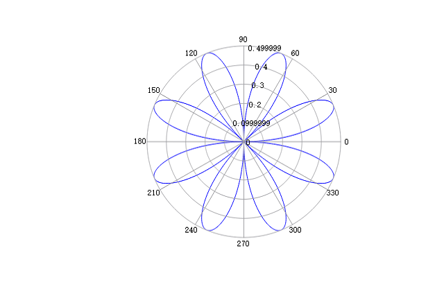
Description
Plots graph in polar coordinates.
Used in FDTD and FDE.

Syntax

Code	Function
`polar(theta, r);`	Plots r versus theta in polar coordinates.
`polar(theta, r, 'line_type');`	Plots r versus theta with specified line style, marker and color designated by 'line_type' in polar coordinates.

Example

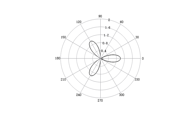
theta = linspace(0, 2*pi, 1000);
r = sin(2*theta).*cos(2*theta);

figure;
polar(theta, r, 'b');

Result:

See also
rlim

smithchart

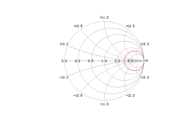
Description
Plots smith chart.
Used in FDTD and FDE.

Syntax

Code	Function
`smithchart(Z);`	Plots a smith chart according to the data Z .
`smithchart(Z, 'line_type');`	Plots a smith chart with specified line style, marker and color designated by 'line_type' according to the data Z .
`smithchart(Z, 'line_type', Z_norm);`	Plots a smith chart with normalized impedance Z_norm. The default impedance used for normalization is 50 Ohms.
`smithchart(Z, 'line_type', Z_norm, equal_aspect_ratio);`	Plots a smith chart with normalized impedance Z_norm (The default impedance used for normalization is 50 Ohms) and equal aspect ratio equal_aspect_ratio.

Example
Plots the simth chart according to the Z data.

Z = 50*(3+1i*linspace(-50, 50, 101)); 

smithchart(Z, 'r');

Result:

See also
polar

surfsph

Description
Draw a radiation map.
This function plots a radiation map. The value F is the value(also color) above the mesh in the theta-phi-R spatial curved surface defined by theta and phi. In particular, R is the 3rd-axis position, not the value(also color).
Used in FDTD and FDE.

Syntax

Code	Function
`surfsph(phi, theta, R);`	Draw a radiation map.The parameters phi, theta, R are the coordinate vector array to set coordinate axis range respectively. F matrix is the module of the three inputs, which is automatically calculated.
`surfsph(phi, theta, R, F)`	Draw a radiation map. The parameters phi, theta, R are the coordinate vector array to set coordinate axis range respectively. And parameter F is field matrix, whose dimensions are the same as ndgrid(phi, theta) or meshgrid(phi,theta).

Example

# theta,phi data
theta = linspace(0, pi, 75);   # theta [0,pi]
phi = linspace(0, 2.*pi, 45);  # phi [0,2*pi]
[T,U] = meshgrid(phi, theta);

n = 10;
psi = pi/2.*(cos(U)-1)-pi/10;
E = sin(pi/2/n).*sin(n.*psi/2)./sin(psi/2);

X = sin(U).*cos(T);
Y = sin(U).*sin(T);
Z = cos(U);

# use surfsph to show iamge 
figure;
surfsph(T, U, abs(E)./abs(E));
title("surfsph-a classical antenna");


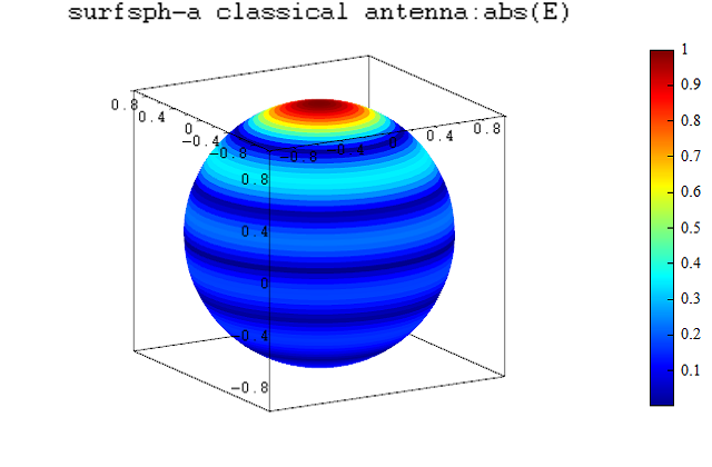
figure;
surfsph(T, U, abs(E)./abs(E),abs(E));
title("surfsph-a classical antenna:abs(E)");

Result:
surfsph-a classical antenna:

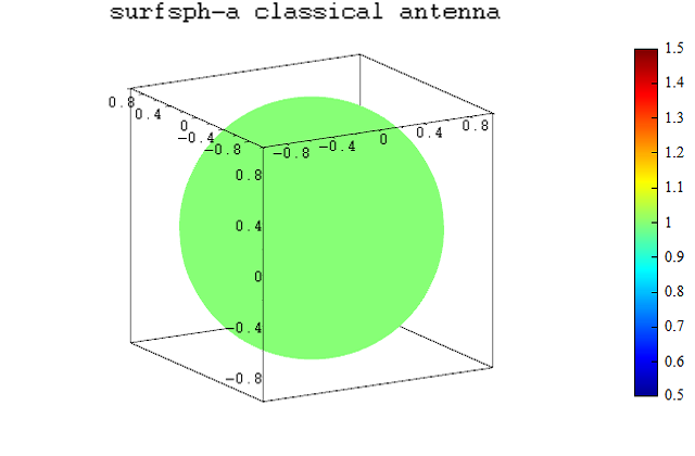
surfsph-a classical antenna:abs(E):

See also
surf, mesh

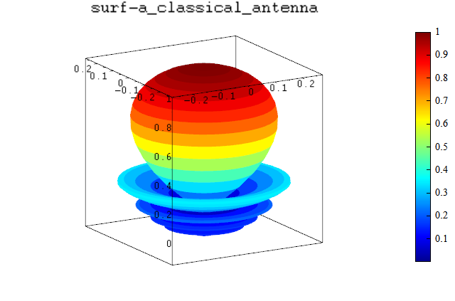
Special note:
Both surf function and surfsph function can draw a radiation plot. The surf function's position inputs x, y, z are defined in Cartesian coordinate system, but surfsph function's position inputs are theta, phi, R in spherical coordinate system.

The following example is used to illustrate the difference between surf function and surfsph function.

numv = 75;
numt = 45;

theta = linspace(0, 1.*pi, numv);  # theta [0,pi]
phi = linspace(0, 2.*pi, numt);    # phi [0,2*pi]
[T,U] = meshgrid(phi, theta);


# a classical antenna
n = 10;
psi = pi/2.*(cos(U)-1)-pi/10;
E = sin(pi/2/n).*sin(n.*psi/2)./sin(psi/2);

# sursph draw 
figure();
surfsph(T, U, abs(E), abs(E));
title('surfsph-a_classical_antenna');

# surf draw
# convert spherical coordinates to Cartesian coordinates
X = sin(U).*cos(T).*abs(E);
Y = sin(U).*sin(T).*abs(E);
Z = cos(U).*abs(E);
figure();
surf(X, Y, Z, abs(E));
title('surf-a_classical_antenna');

Result:
surfsph-a_classical_antenna:

surf-a_classical_antenna:

Graphics Formatting

figure

Description
Creates a new figure window.
Used in FDTD and FDE.

Syntax

Code	Function
`figure;`	Creates a new figure window using default property values. The resulting figure is the current figure.
`figure(id);`	Creates a new figure window specified by id as the current figure window and displays it on top of all other figures.

See also
plot

subplot

Description
Divides a single figure into multiple subareas and specifies the area where the graph will be drawn.
Used in FDTD and FDE.

Syntax

Code Function

subplot(m, n, index); Divides the current figure into an m * n grid of subplot areas, and then specifies the area to be used for drawing by the input parameter index . The index of subplot area starts at 1 in the first column of the first row and increases to the right. The index of the subplot area in the first column of the first row is 1, the index of the subplot area in the second column of the first row is 2, and so on.

Code	Function
`subplot(m, n, index);`	Divides the current figure into an m * n grid of subplot areas, and then specifies the area to be used for drawing by the input parameter index . The index of subplot area starts at 1 in the first column of the first row and increases to the right. The index of the subplot area in the first column of the first row is 1, the index of the subplot area in the second column of the first row is 2, and so on.

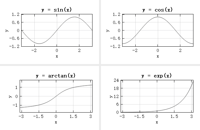
Example

This example aims to display four different functions in the same figure. For each function, the subplot function is used to designate the area where the function is to be plotted, after which the function is drawn.

x = linspace(-pi, pi, 1000);

figure;
subplot(2, 2, 1);
plot(x, sin(x));
xlabel('x');
ylabel('y');
title('y = sin(x)');

subplot(2, 2, 2);
plot(x, cos(x));
xlabel('x');
ylabel('y');
title('y = cos(x)');

subplot(2, 2, 3);
plot(x, atan(x));
xlabel('x');
ylabel('y');
title('y = arctan(x)');

subplot(2, 2, 4);
plot(x, exp(x));
xlabel('x');
ylabel('y');
title('y = exp(x)');

Result:

See also
figure, plot, image

xlabel

Description
Sets the label for x axis.
Used in FDTD and FDE.

Syntax

Code	Function
`xlabel('x_label');`	Sets the x axis label of current figure as 'x_label' .
`xlabel(fig_id, 'x_label');`	Sets the x axis label of figure designated by fig_id as 'x_label' .

Example
Plots a sine function and sets the x axis label as 'x'.

# prepare data
pi = 3.1415926;
x = linspace(0, 2*pi, 100);
y = sin(x); 

# plot sine function
figure; 
plot(x, y, 'r');
xlabel('x');

Result :

See also
ylabel, title, figure, plot

ylabel

Description
Sets the label for y axis.
Used in FDTD and FDE.

Syntax

Code	Function
`ylabel('y_label');`	Sets the y axis label of current figure as 'y_label'.
`ylabel(fig_id, 'y_label');`	Sets the y axis label of figure designated by fig_id as 'y_label'.

Example
Plots a sine function and sets the y axis label as 'y'.

# prepare data
pi = 3.1415926;
x = linspace(0, 2*pi, 100);
y = sin(x); 

# plot sine function
figure; 
plot(x, y, 'r');
ylabel('y');

Result :

See also
ylabel, title, figure, plot

title

Description
Sets title for the figure.
Used in FDTD and FDE.

Syntax

Code	Description
`title('fig_title');`	Sets title for current figure,
`title(fig_id, 'fig_title')`	Sets the title for the figure designated by fig_id .

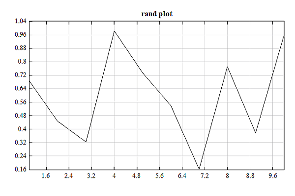
Example

figure;
plot(rand(1, 10));
title('rand plot');

Result:

See also
xlabel, ylabel, legend

legend

Description
Adds a legend to a line plot.
Used in FDTD and FDE.

Syntax

Code	Description
`legend('legend1', 'legend2', ..., 'legendn' );`	Sets the legend labels for each line, each parameter is string.
`legend(legend_array);`	Sets the legend using a cell array or a character matrix.

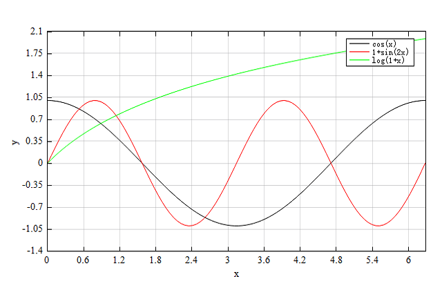
Example
Plot three different functions and add legend for them.

# prepare data
x = linspace(0,2*pi);
y1 = cos(x);
y2 = sin(2*x);
y3 = log(1+x);

# plot 
figure;
plot(x, y1);
hold_on;
plot(x, y2);
hold_on;
plot(x, y3)
xlabel('x');
ylabel('y');
legend('cos(x)', '1+sin(2x)', 'log(1+x)');

Result:

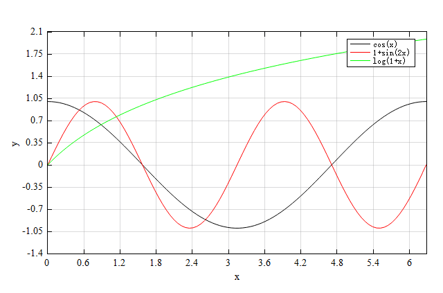
Use cell to set legend.

# prepare data
x = linspace(0, 2*pi);
y1 = cos(x);
y2 = sin(2*x);
y3 = log(1+x); #log is the natural logarithm function.

# cell to set legend
legend_cell={'cos(x)','1+sin(2x)','log(1+x)'};

# plot 
figure;
plot(x, y1);
hold_on;
plot(x, y2);
hold_on;
plot(x, y3);
xlabel('x');
ylabel('y');
legend(legend_cell);

Result:

See also
xlabel, ylabel

xlim

Description
Sets x-axis limits, supports figure of plot and image.
Used in FDTD and FDE.

Syntax

Code	Description
`xlim(x_lim);`	Sets the x-axis limits for the current figure with the specified number. The parameter x_lim must be a two-element vector of the form [x_min, x_max], where x_max is a numeric value greater than x_min.
`xlim(fig_id, x_lim);`	Sets the x-axis limits for figure specified by fig_id with the specified number.

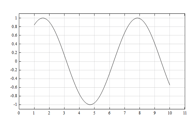
Example

x=linspace(1, 10, 100);
y=sin(x);

figure;
plot(x, y);
xlim([0, 11]);

Result:

See also
ylim

ylim

Description
Sets y-axis limits, supports figure of plot and image.
Used in FDTD and FDE.

Syntax

Code	Description
`ylim(y_lim);`	Sets the y-axis limits for the current figure with the specified number. The parameter y_lim must be a two-element vector of the form [y_min, y_max], where y_max is a numeric value greater than y_min.
`ylim(fig_id, y_lim);`	Sets the y-axis limits for figure specified by fig_id with the specified number.

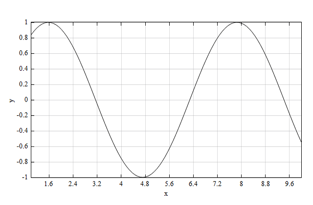
Example

x=linspace(1, 10, 100);
y=sin(x);

figure;
plot(x, y);
ylim([-1, 1]);
xlabel('x');
ylabel('y');

Result:

See also
xlim

y2lim

Description
Sets y2-axis limits, supports figure of plot and image.
Used in FDTD and FDE.

Syntax

Code	Function
`y2lim(y2_lim);`	Sets the y2-axis limits for the current figure with the specified number. The parameter y2_lim must be a two-element vector of the form [y2_min,y2_max], where y2_max is a numeric value greater than y2_min.
`y2lim(fig_id, y2_lim);`	Sets the y2-axis limits for the figure with the specified number.

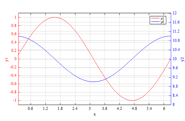
Example

x=linspace(0.1, 2*pi, 100);
y1 = sin(x);
y2 = 10 + cos(x);

figure;
plotyy(x, y1, x, y2);
y2lim([8, 12]);
legend('y1', 'y2');
xlabel('x');
ylabel('y1');
ylabel2('y2');

Result:
img/y2lim_example_y1_y2.png
See also
ylim, xlim

ylabel2

Description
Sets label for second y axis.
Used in FDTD and FDE.

Syntax

Code	Description
`ylabel2('y2_label');`	Sets the y2 axis label of current figure as 'y2_label'.
`ylabel2(fig_id, 'y2_label')`	Sets the y2 axis label of figure designated by fig_id as 'y2_label'.

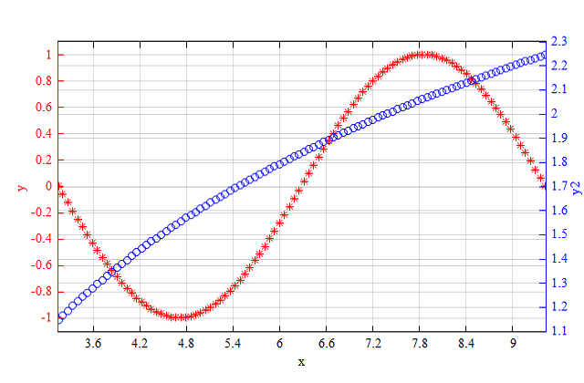
Example

x=linspace(pi,3*pi);
y1 = sin(x);
y2 = log(x); # natural logarithm function

figure;
plotyy(x, y1, x, y2, '*r', 'ob');
ylabel('y');  # set y1 axis label
ylabel2('y2'); # set y2 axis label
xlabel('x');

Result:

See also
xlabel

rlim

Description
Sets the r-axis limits, supports figure of polar.
Used in FDTD and FDE.

Syntax

Code	Function
`rlim(r_lim);`	Sets the r-axis limits for the current polar figure with the specified number. The parameter r_lim must be a two-element vector of the form [r_min, r_max], where r_max is a numeric value greater than r_min.
`rlim(fig_id, limit);`	Sets r-axis limits for the polar figure designated by fig_id with specified number. The parameter r_lim must be a two-element vector of the form [r_min, r_max], where r_max is a numeric value greater than r_min.
`rlim('auto');`	Sets the r-axis limits back to the original values.

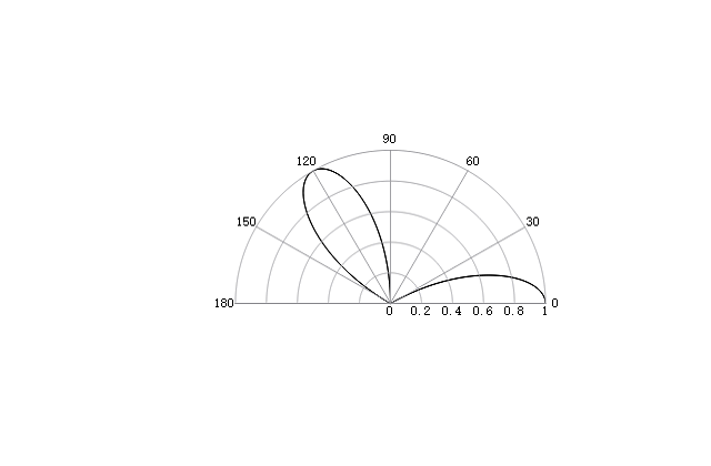
Example
Create a polar plot and change the r-axis limits.

phi = linspace(0, 2*pi, 500);
r = cos(3*phi);

figure;
polar(phi, r);
rlim([0, 2]);

Result:

See also
thetalim

thetalim

Description
Sets theta-axis limits,supports figure of polar.
Used in FDTD and FDE.

Syntax

Code	Description
`thetalim(theta_lim);`	Sets theta-axis limits for the current polar figure with the specified number. The parameter theta_lim must be a two-element vector of the form [theta_min, theta_max], where theta_max is a numeric value greater than theta_min.
`thetalim(fig_id, theta_limit);`	Sets theta-axis limits for the polar figure designated by fig_id with specified number. The parameter theta_lim must be a two-element vector of the form [theta_min, theta_max], where theta_max is a numeric value greater than theta_min.
`thetalim('auto');`	Sets the theta-axis limits back to the original values.

Example
Create a polar plot and change the theta-axis limits.

phi = linspace(0, 2*pi, 500);
r = cos(3*phi);

figure;
polar(phi, r);
thetalim([0, 180]);

Result:

See also
rlim

zlabel

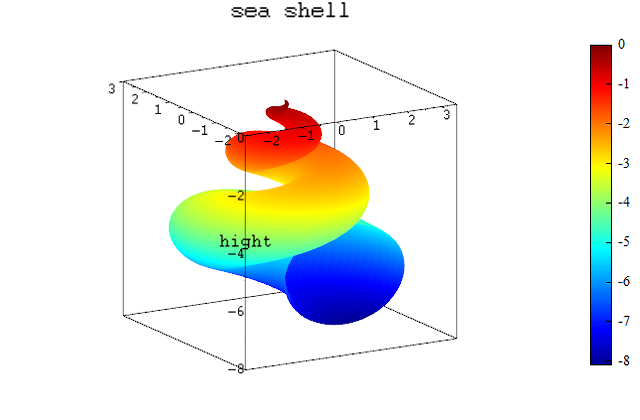
Description
Sets the z-axis label for surf, surfsph, vectorplot figure.
Used in FDTD and FDE.

Syntax

Code	Function
`zlabel('z_label');`	Sets the z-axis label of current `surf`, `surfsph` or `vectorplot` figure as z_label.
`zlabel(fig_id, 'z_label');`	Sets the z-axis label of `surf`, `surfsph` or `vectorplot` figure designated by fig_id as z_label.

Example

# prepare data
a = 2;
b = 6*pi;
c = 3*pi;

u0 = linspace(0, b, 300);
v0 = linspace(0, c, 300);
[u,v] = meshgrid(u0,v0);

X = a.*(exp(u./b)-1).*cos(u).*(cos(v/2)).^2;
Y = a.*(1-exp(u./b)).*sin(u).*(cos(v/2)).^2;
Z = exp(u./b).*sin(v)-exp(u./c)-sin(v)+1;

# show image
figure();
surf(X, Y, Z, Z);
zlabel('hight');
title('sea shell');

Result:

See also
xlabel, ylabel

holdon

Description
Maintains the plot in the current figure so that the new plot can be added to the current figure together.
Used in FDTD and FDE.

Syntax

Code	Function
`holdon;`	Maintains the plot in the current figure so that the new plot can be added to the current figure together.

See also
holdoff

holdoff

Description
Clears the plot in the current figure and reset the figure properties so that the new plot can be shown in the current figure alone.
Used in FDTD and FDE.

Syntax

Code	Function
`holdoff;`	Clears the plot in the current figure and reset the figure properties so that the new plot can be shown in the current figure alone.

See also
holdon

close

Description
Closes the specified figure window.
Used in FDTD and FDE.

Syntax

Code	Function
`close;`	Closes the current figure window.
`close(id);`	Closes the figure window designated by id .

Example

figure;
plot(rand(1,3));
close; # close current figure window

See also
closeall

closeall

Description
Closes all the figure windows.
Used in FDTD and FDE.

Syntax

Code	Function
`closeall;`	Closes all the figure windows.

Example

figure;
plot(rand(1,3));
 
figure;
plot(rand(1,3));
 
closeall; # close all the figure windows

See also
close