This section introduces the functions used in the numerical integration & difference, interpolation, and Fourier analysis.

diff

Description
1-order nD difference.
Used in FDTD and FDE.

Syntax

Code	Function
`v = diff(D);`	If D is a vector, returns the vector whose elements are the difference between the adjacent element of D. If D is a matrix, returns a matrix whose elements are the differences between the rows of D.
`v = diff(D, N);`	Returns a vector or matrix containing the N th difference of D by applying the `diff(D)` operation for N times.

See also
integrate

integrate

Description
Calculates nD integral.
Used in FDTD and FDE.

Syntax

Code	Function
`I = integrate(A, n, x1);`	Calculates the integral in the specified dimension of A designated by n according to the corresponding position vector x1 for that dimension.
`I = integrate(A, d, x1, x2, ...);`	Calculates the integral in the specified dimensions of A designated by vector d respectively according to the corresponding position vectors x1, x2, ... for those dimensions.

Example

Example 1:

Calculates the integral of input 2D data.


y=[1,2,3;4,5,6];

# (2.5-1)*0.5*1+(2.5-1)*0.5*4
# (2.5-1)*0.5*2+(2.5-1)*0.5*5
# (2.5-1)*0.5*3+(2.5-1)*0.5*6
r = integrate(y,1,[1,2.5])

Result:

Example 2:
Calculates multiple dimensions of integral.

y=zeros(2,3,2,2);

y(:,:,1,1) = [1,2,3;4,5,6];
y(:,:,2,1) = [7,8,9;10,11,12];
y(:,:,1,2) = [13,14,15;16,17,18];
y(:,:,2,2) = [19,20,21;22,23,24];


# integrate first and third dimension
r = integrate(y, [1,3], [1,2], [1,4])

Result:

r =
          16.5          52.5
          19.5          55.5
          22.5          58.5

interp

Description
Calculates linear interpolation.
Used in FDTD and FDE.

Syntax

Code	Function
`interp(D, x, x1);`	Calculates 1D linear interpolation in new coordinates x1 according to old data D and old coordinates x.
`interp(D, x, y, x1, y1);`	Calculates 2D linear interpolation in new coordinates x1, y1 according to old data D and old coordinates x, y.
`interp(D, x, y, z, x1, y1, z1);`	Calculates 3D linear interpolation in new coordinates x1, y1, z1 according to old data D and old coordinates x, y, z.
`interp(D, x, y, z, t, x1, y1, z1, t1);`	Calculates 4D linear interpolation in new coordinates x1, y1, z1, t1 according to old data D and old coordinates x, y, z, t.

Example


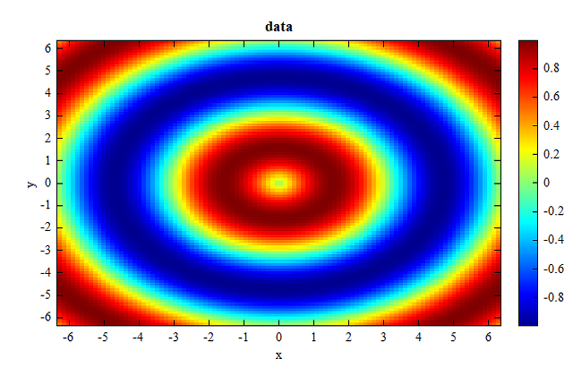
# 2D linear interpolation
x = linspace(-2*pi, 2*pi, 100);
y = linspace(-2*pi, 2*pi, 100);
data = zeros(length(y), length(x));

for (i = 1:length(x))
        for (j = 1:length(y))
                data(j, i) = sin(sqrt(x(i)^2 + y(j)^2));
        end
end

figure();
image(x, y, data);
xlabel('x');
ylabel('y');
title('data');


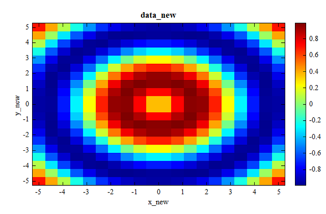
x_new = linspace(-5, 5, 20);
y_new = linspace(-5, 5, 20);
data_new =interp(data, x, y, x_new, y_new);

figure();
image(x_new, y_new, data_new);
xlabel('x_new');
ylabel('y_new');
title('data_new');

Result:
data(initial data):

new data:

fft

Description
Fast Fourier Transform Algorithm.
Used in FDTD and FDE.

Syntax

Code	Function
`v = fft(D);`	Calculates the discrete Fourier transform (DFT) of D using a fast Fourier transform (FFT) algorithm.
`v = fft(D, N, dim);`	Calculates the N point discrete Fourier transform (DFT) of D using a fast Fourier transform (FFT) algorithm.
`v = fft(D, N, dim);`	Calculates the N point discrete Fourier transform (DFT) of D along the dimension designated by dim using a fast Fourier transform (FFT) algorithm.

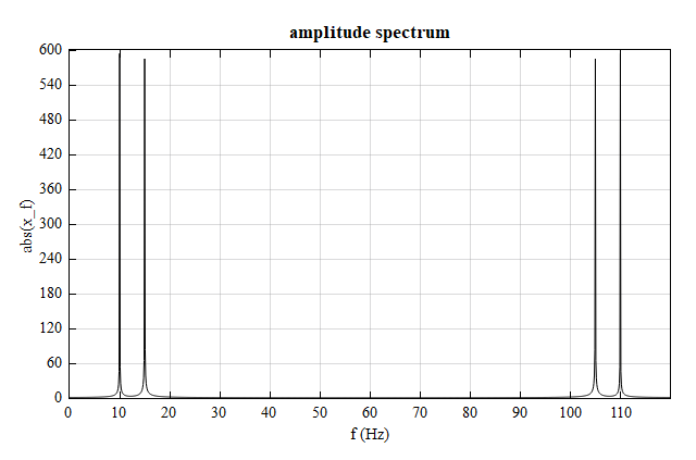
Example

f1 = 10;     # frequency in Hz
f2 = 15;
fs = 120;    # sampling frequency in Hz
Ts = 1/fs;   # sampling period
t = -5:Ts:5;
L = length(t);

# time signal
x_t = cos(2*pi*f1*t) + sin(2*pi*f2*t);

# frequency spectrum
x_f = fft(x_t);

# frequency vector
f = 0:1:(L-1);
f = f*(fs/L); 

# plot amplitude spectrum
figure;
plot(f, abs(x_f));
xlabel('f (Hz)');
ylabel('abs(x_f)');
title('amplitude spectrum');

Result(amplitude spectrum):

See also
fftshift

fftshift

Description
Shifts zero frequency component to center of spectrum.
Used in FDTD and FDE.

Syntax

Code	Function
`v = fftshift(D);`	Shifts zero frequency component to center of spectrum for D.
`v = fftshift(D, dim);`	Shifts zero frequency component to center of spectrum for D along the designated dimension dim.

Example

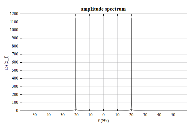
f0 = 20;     # frequency in Hz
fs = 120;    # sampling frequency in Hz
Ts = 1/fs;   # sampling period
t = 0:Ts:20;
L = length(t);

# time signal
x_t = sin(2*pi*f0*t) ;

# frequency spectrum  
x_f = fftshift( fft(x_t) );
L_h = (L-1)./2;

# frequency vector 
f = -L_h:1:L_h;
f = f * fs /L;

# plot amplitude spectrum
figure;
plot(f, abs(x_f));
xlabel('f (Hz)');
ylabel('abs(x_f)');
title('amplitude spectrum');

Result(amplitude spectrum):

See also
fft

fft2

Description
Two-dimensional Fourier Transform.
Used in FDTD and FDE.

Syntax

Code	Function
`f = fft2(x);`	Returns the two-dimensional Fourier transform matrix with the same dimension as the matrix x.
`f = fft2(x, mrows, ncols)`	Returns the two-dimensional Fourier transform matrix with designated dimension ( mrows, ncols ).

See also
fft

ifft

Description
Inverse Fast Fourier Transform Algorithm.
Used in FDTD and FDE.

Syntax

Code	Function
`v = ifft(D);`	Returns the inverse Fourier transform matrix with the same dimension as the matrix D.
`v = ifft(D, N);`	Calculates the N point inverse discrete Fourier transform (DFT) of D by using inverse fast Fourier transform algorithm.

See also
fft2

ifft2

Description
Two-dimensional Inverse Fourier Transform.
Used in FDTD and FDE.

Syntax

Code	Function
`f = ifft2(x);`	Returns the two-dimensional inverse Fourier transform matrix with the same dimension as the matrix x.
`f = ifft2(x, mrows, ncols);`	Returns the two-dimensional inverse Fourier transform matrix with designated dimension ( mrows, ncols ).

See also
fft

fftw

Description
Transforms a frequency vector from the input time vector.
Used in FDTD and FDE.

Syntax

Code	Function
`f = fftw(t, zero_pad);`	Returns the angular frequency vector of time vector t. The parameter zeros_pad determines the number of elements in the frequency vector.

Note:
When the length of time vector is larger than zero_pad, zero_pad is exchanged as a new number, also an power of 2, up to the next power of 2 longer than the length of time; when the interval of the time is not an equal-radio data, also could calculate.

Example

t = [0.1, 1.1, 2.1, 3.1, 4.1, 5.1, 6.1, 7.2, 8.1, 9.1];
zero_pad  = 2^4;
w  = fftw(t,zero_pad);

Result:

w =
 columns 1 through 8
             0   0.392699082   0.785398163    1.17809725    1.57079633    1.96349541    2.35619449    2.74889357

 columns 9 through 16
    3.14159265    3.53429174    3.92699082     4.3196899    4.71238898    5.10508806    5.49778714    5.89048623

See also
fft

dft

Description
Calculates the discrete fourier transform.
Used in FDTD and FDE.

Syntax

Code	Function
`f = dft(D, frequency_point, delta_time, frequency_length) ;`	Calculates the discrete fourier transform of D in designated frequency point and length with delta time delta_time.

See also
fft

czt

Description
Computes the 1D or 2D chirped z-transform ( or inverse chirped z-transform ) for the defined signal.
Used in FDTD and FDE.

Syntax

Code	Function
`z = czt(signal, pos, pos_trans, type );`	If type is 1, computes the 1D chirped z-transform of the defined signal signal . The input signal signal is a function of the independent variable pos ( usually time ) and pos_trans is the transform domain positions ( usually angular frequency in frequency domain ). If type is not 1, iczt ( inverse chirped z-transform ) will be operated.
`z = czt(signal, xpos, ypos, xpos_trans, ypos_trans, type);`	If type is 1, computes the 2D chirped z-transform of the defined signal signal . The input signal signal is a function of the independent variables xpos and ypos. And xpos_trans, ypos_trans are the transform domain postions. If type is not 1, iczt ( inverse chirped z-transform ) will be operated.

Example

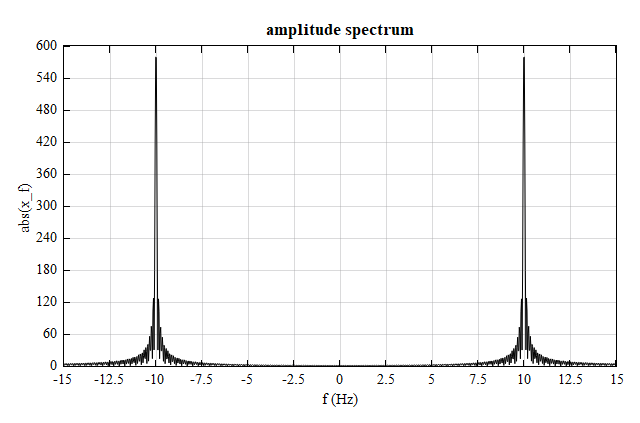
clear;
clc;

f0 = 10;     # frequency in Hz
fs = 120;    # sampling frequency in Hz
Ts = 1/fs;   # sampling period
t = -5:Ts:5;


# time signal
x_t = cos(2*pi*f0*t);

# frequency 
f = linspace(-15, 15, 1000);
w = f*2*pi;

# frequency spectrum
x_f = czt(x_t, t, w);

# plot amplitude spectrum
figure;
plot(f, abs(x_f));
xlabel('f (Hz)');
ylabel('abs(x_f)');
title('amplitude spectrum');

Result(amplitude spectrum):

See also
fft

czt1d

Description
Computes the 1D chirped z-transform(or inverse chirped z-transform) for the defined signal.
Used in FDTD and FDE.

Syntax

Code	Function
`czt1d(x_t, t, omega, type);`	If type is 0, calculates the 1D chirped z-transform of time signal x_t at each desired angular frequency omega . The input signal x_t is a function of the independent variable t (usually time) and omega is angular frequency in frequency domain. If type is not 0, iczt(inverse chirped z-transform) will be operated.

See also
czt

filter

Description
Calculates discrete time recursive filter.
Used in FDTD and FDE.

principle:
filter is an implementation of the standard difference equation:

$y[n] = b(1)*x[n] + b(2)*x[n-1] + ... + b(z+1)*x[n-z] \\ - a(2)*y[n-1] - a(p+1)*y[n-p]$

The filter is implemented using a method described as a 'Direct Form II Transposed' filter. More for information see Chapter 6 of 'Discrete-Time Signal Processing' by Oppenheim and Schafer.

Syntax

Code	Function
`out = filter( B, A, X );`	Implements a discrete time recursive filter according to parameters B, A, X. The meanings of the parameters can be seen below.
`out = filter( B, A, X, Zi );`	Implements a discrete time recursive filter according to parameters B, A, X, Zi. The meanings of the parameters can be seen below.

The inputs to filter are:

B
The numerator coefficients, or zeros of the system transfer function. The coefficients are specified in a vector like:
[ b(1) , b(2) , ... b(z) ]
A
The denominator coefficients, or the poles of the system transfer function. The coefficients are specified in a vector like:
[ a(1) , a(2) , ... a(p) ]
X
A vector of the filter inputs.
Zi
[Optional] The initial delays of the filter.
The filter outputs are in a list with element names:
y
The filter output. y is a vector of the same dimension as X.
zf
A vector of the final values of the filter delays.

Note:
The a(1) coefficient must be non-zero, as the other coefficients are divided by a(1).

Example

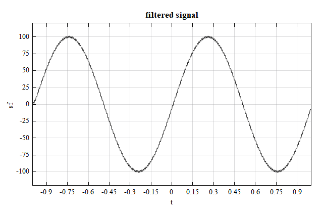
Below is an implementation of a simple lowpass filter using the filter function. The lowpass filter depends on the following difference equation:

$y[n] = \frac{1}{1+ T_{s}\omega_{c}}y[n-1] + \frac{T_{s}\omega_{c}}{1+ T_{s}\omega_{c}}x[n]$

clear;
clc;

fs = 1000;      # sample frequency
Ts = 1/fs;      # sample period
w1 = 2*pi;
w2 = 100*2*pi;
wc = 100;


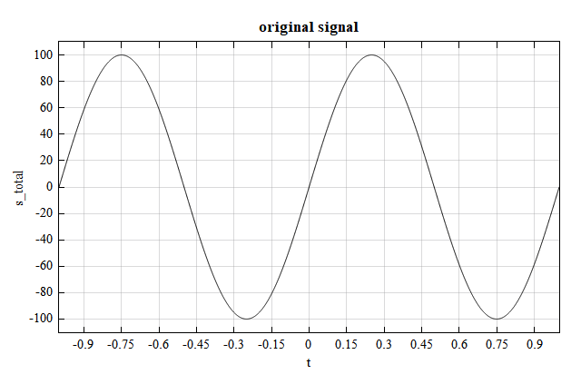
t = -1:Ts:1;

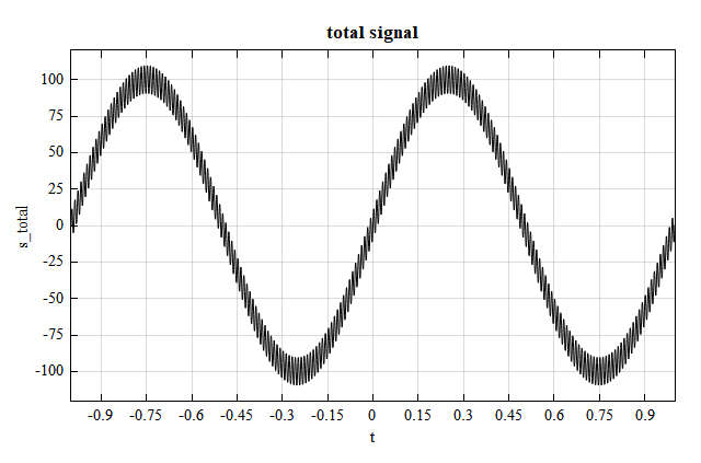
s1 = 100*sin(w1*t); # original signal
sn = 10*sin(w2*t);  # high frequency noise
s_total = s1 + sn;

cf = 1/(1 + Ts*wc);
a = [1, -cf];
b = 1 - cf;

sf = filter(b, a, s_total);



figure;
plot(t, s1);
xlabel('t');
ylabel('s_total');
title('original signal')


figure;
plot(t, s_total);
xlabel('t');
ylabel('s_total');
title('total signal')

figure;
plot(t, sf.y);
xlabel('t');
ylabel('sf');
title('filtered signal');

Result:
original signal:

total signal:

filtered signal: