宽带仿真中的模式源
前言
在默认情况下,模式光源使用频域算法计算中心频点处结构中稳定存在的模式分布,然后在所有频率范围内注入该模式。这种方法在单频和窄带仿真中非常有效,但是在宽带仿真中,如果结构中对于不同频率的模场分布差别很大,那么模式不匹配的误差就会随着频率范围的增大而增大。因此在宽带仿真中建议使用多频点解模来减少模式不匹配的误差。本文将以在宽带太赫兹范围内工作的带有薄介电涂层的铜线为例,演示模式源的多频解模功能。仿真模型如下图所示,注入脉冲将会以表面波的形式沿着导线传播,并产生啁啾信号。且由于铜线表面的介电涂层导致注入模式具有色散性,因此模式分布随频率而发生巨大变化,非常适合展示多频点模式源在宽带仿真中的优势。
仿真设置
模型简介
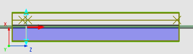
本案例中,我们使用完美电导体(PEC)材料来模拟铜线,铜线的半径为 。在铜线的外面还有一层厚度为 、折射率为 的介电涂层,模式源从铜线的左侧垂直入射,如上图。由于结构以及光源的对称性质,我们可以在 方向上使用Symmetric对称边界条件。使用对称边界条件可以将仿真区域缩小至1/2,从而减少仿真所需要的内存。
光源设置
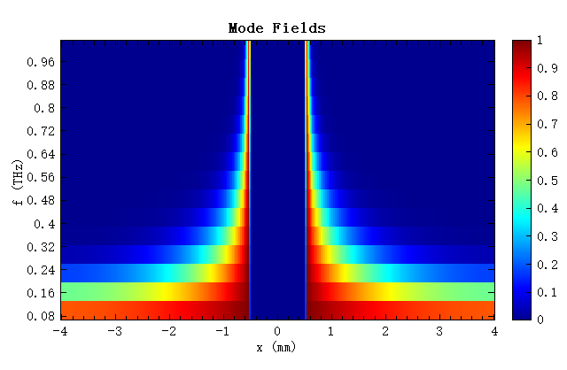
本案例中,铜线工作带宽为 ,如果使用默认的模式光源(单频点解模)会由于模式不匹配带来很大的误差。因此我们需要勾选模式源的multi-frequency field多频解模功能,并设置频点数为15。解模完成后可以查看模式场剖面随频率变化的分布图,如下图。从图中可以看到,在该仿真中模式场随频率的变化非常大。
仿真结果
运行附件中的 Broadband_modesource_wire_multifreq.msf 脚本,脚本会自动设置并运行一个使用默认模式源的仿真工程和一个使用多频点解模模式源的工程。
使用默认模式源时,注入脉冲、传播至铜线右侧的脉冲以及后向散射的脉冲随时间变化图如下:
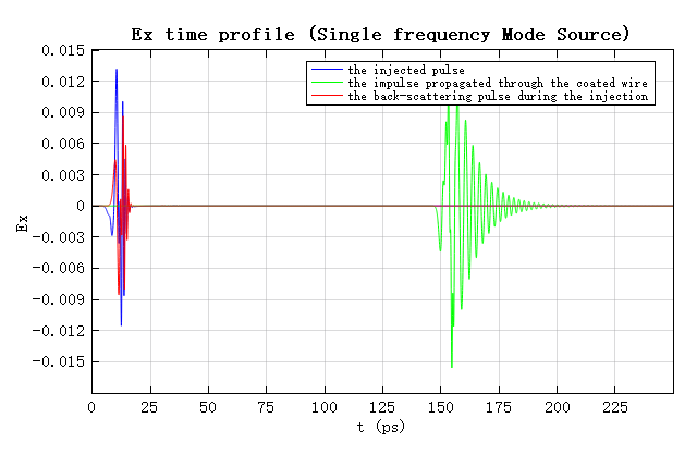
可以清楚地看到,中心频率求解的模式与整个频段的模式不匹配,导致产生大量的后向散射。注入脉冲与后向散射相互干扰,信号很不清晰。
下图为开启多频解模功能后,模式源的注入脉冲、传播至铜线右侧时的脉冲以及注入时产生的后向散射的脉冲随时间变化的图。
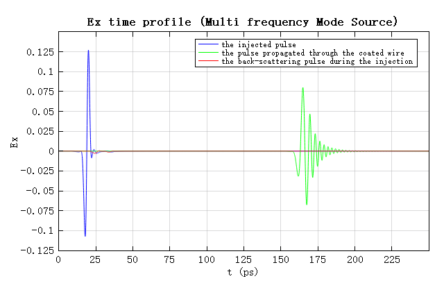
从图中可以看出,注入脉冲的时域场非常清晰,几乎没有产生后向散射。注入脉冲沿着铜线传播至右侧时由于色散产生的啁啾信号也非常干净。
相关视频