使用非线性材料产生谐波
前言
在非线性光学中,光与介质相互作用产生了非线性极化,光的电场分量 E 与非线性极化强度 P 的关系为:
其中 、 、 分别为介质的线性极化率、二阶非线性极化率、三阶非线性极化率。忽略三阶以及更高阶项,该式即为二阶非线性材料极化强度的表达式。二阶非线性效应在光学倍频、混频、调制等领域应用广泛,在激光器、频率转换等器件当中扮演着重要作用。本案例将利用二阶非线性材料仿真二次谐波的产生。
仿真设置
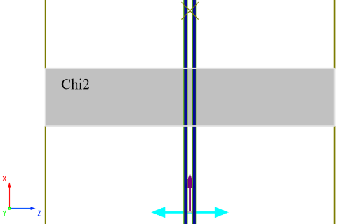
本案例使用 2D FDTD 进行仿真,平面波光源入射到非线性材料 chi2 中,并在材料后方接收其透射的光谱信息。其结构如下图所示,在 z 方向上使用Periodic边界条件,以得到该方向上无限大的仿真结果。
在材料库当中定义二阶非线性材料 chi2 时,需要设置Base Material和非线性极化系数,未选择基底材料时,默认折射率为 1,具体细节可参考Nonlinear Material。其非线性极化系数应当满足下式
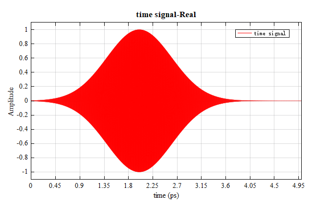
在非线性仿真当中,光源的脉冲形状是非常重要的,本案例在Time Domain当中设置自定义的脉冲信号,如下图所示,同时,增大光源的振幅,以得到更理想的非线性效应。
值得注意的是,仿真当中需要关闭Continuous Wave Normalization功能,开启该功能时,将会利用光源时间脉冲的傅里叶变换对接收到的场进行归一化处理,从而得到系统的频域响应,但该过程仅对线性效应是完全正确的。
在默认非均匀网格下,网格尺寸会根据仿真光源的范围自动计算,但是由于忽略了非线性效应产生的高频分量,会导致网格细化地不够充分。我们使用override bandwidth for mesh generation设置,选择自定义的波长范围(包括非线性产生的短波长)来重新划分网格,使得网格划分能够满足仿真需求。而在TimeMonitor当中,为防止对非线性效应产生的高频分量采样不足导致的频率重叠,应适当增加默认的采样点数。
仿真结果
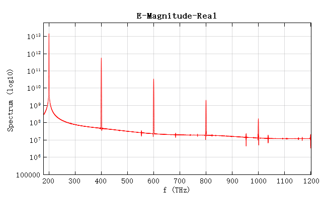
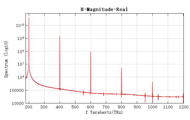
打开附件,直接运行,在时间监视器当中可以得到经过傅里叶变化的频谱(见下图)。结果表明接收的光谱不仅仅在光源 200THz 附近存在共振峰,在后续 400、600、800THz 处也产生了共振峰,表明光与非线性材料相互作用时,产生了二次谐波。