高Q腔的场幅值校正
前言
品质因子 Q 值的定义为中心谐振波长与谐振峰半高全宽的比值,Q 值越高,表明器件对波长的选择性越好,输出峰值越陡峭,器件的灵敏度越高。一般在高 Q 值谐振腔的仿真中,得到的场幅值是不准确的。原因是高 Q 值谐振腔的损耗速度慢,若仿真时间不够长时,腔内的场在仿真结束时仍未衰减为 0。此时需要对腔内模式场的幅值进行校正才能得到模式最终在腔内的实际幅值。本案例构建了光子晶体谐振腔结构,展示如何在高 Q 值谐振腔仿真时间不够时校正场的幅值。
仿真设置
模型构建
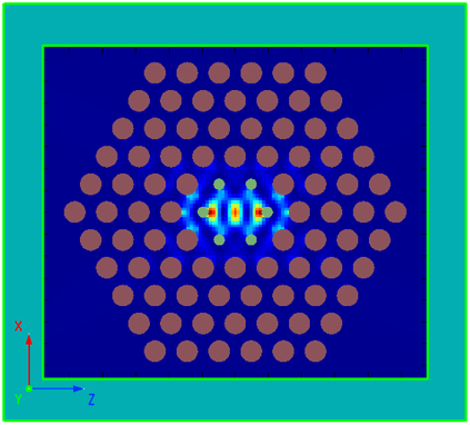
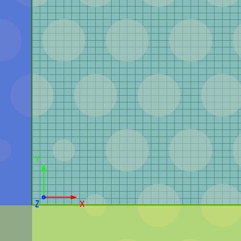
本案例中使用的谐振腔为一个具有六角晶格空气孔的氧化钽( )。在光子晶体结构的仿真中,网格的划分非常重要,需要保证每个周期结构单元的网格剖分方式相同。本案例中通过添加均匀覆盖网格来确保正确的周期单元分布。由于结构与光源的对称性,在 方向上使用Symmetric对称边界条件,在 方向上使用Anti-Symmetric反对称边界条件。使用对称/反对称边界条件可以将仿真区域缩小至 1/8,从而减少仿真需要的内存。
校正场幅值
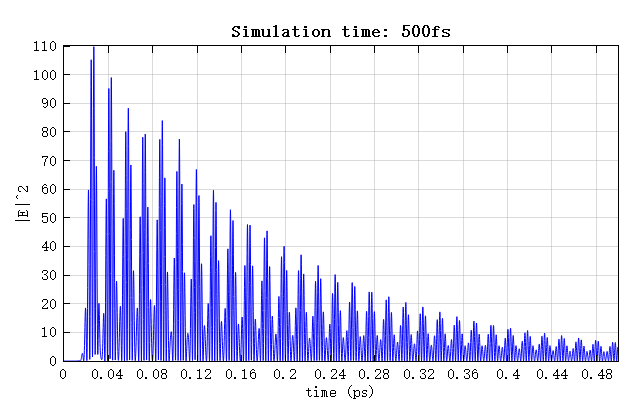
绝对模式场描述了模式场的空间形状以及源和空腔模式之间的耦合强度。由于FDTD中使用的光源并不代表用于激发空腔的实际光源,因此绝对模式场通常并不是一个值得关注的量,质量因子 Q 和相对模式场分布通常才是我们感兴趣的量。但如果您在FDTD中使用的光源就是实际激发空腔的源,您可能希望了解模式场的实际振幅。如下图所示,高 Q 值空腔的模式振幅不准确的原因是模拟在空腔场衰减为 0 之前就结束了,只有在考虑整个时间信号时,FDFP监视器计算的结果才是正确的。

通过对模拟出的原始场的幅值进行放缩,就可以校正出绝对场幅值。场的幅值与上图中曲线下的面积成正比,因此可根据仿真时间对应的面积比例来校正幅值。场幅值的比例因子同时由谐振频率 、仿真结束时间 和模式质量因子 决定,可由下式表示。
因此,我们只需要使用high Q analysis分析组计算出该空腔的 Q 值就可以得到原始场幅值的放缩比例,从而校正出绝对场幅值。
仿真结果
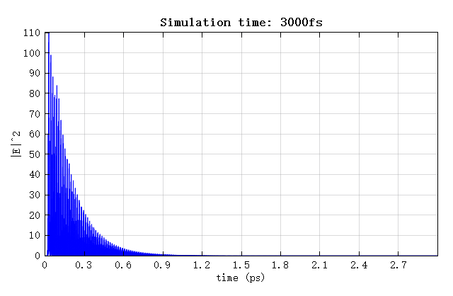
运行附件中的脚本文件可以自动运行两个仿真时长分别为 500fs 和 3000fs 的模拟。下图为两次模拟中,时间监视器得到的电场强度随仿真时间的分布图。从图中可以看出,当 500fs 的模拟时间不足以让场完全衰减,所以最终得到的场幅值是不准确的,需要通过校正来弥补较短的仿真时长。
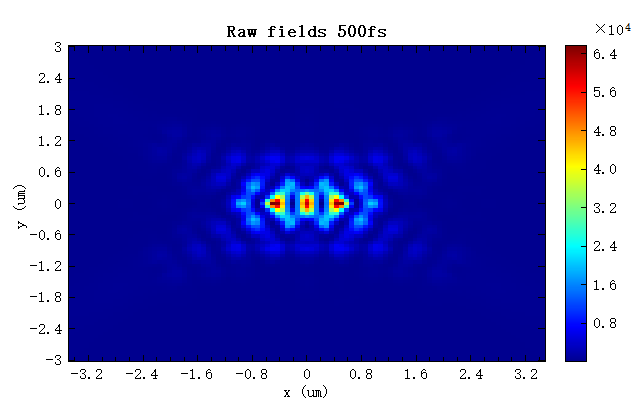
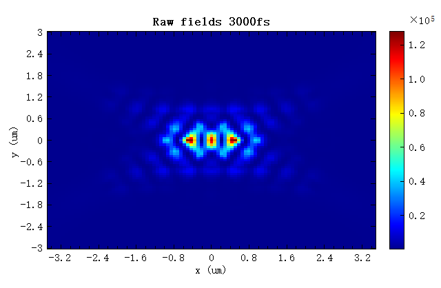
下图为FDFP监视器中得到的谐振腔内原始的场分布。请注意,腔内的场幅值取决于仿真时长。如果仿真时间不够长,场幅值就会小于应有的值。从图中可以看出仿真时长为 500fs 时,场幅值明显小于仿真时长为 3000fs 时的幅值。
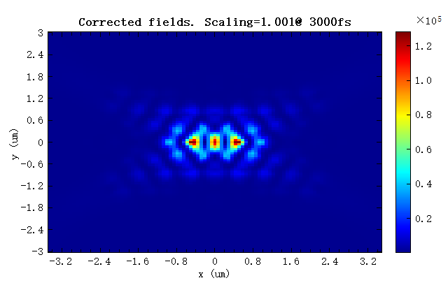
下图为经过幅值校正后,500fs 和 3000fs 仿真时间得到的电场强度分布,不同仿真时长得到的场幅值经校正后得到基本一致的数值。可以看到 500fs 模拟的场被放大了,以补偿模拟时间的缩短,3000fs 仿真时间得到场比例因子约等于 1。如果模拟运行的时间足够长,场完全衰减,则无需重新缩放场,比例因子应等于 1。

注意,虽然仿真时长不同,但计算得到的 Q 值是相同的,这是因为两个仿真中获取的场分布是相同的。所以不需要让仿真持续到场完全衰减。所有的信息都可以从较短的仿真中获取。