同轴馈电矩形贴片天线
前言
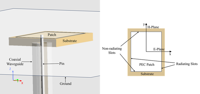
贴片天线是最基本的微带天线,由介质基板、接地板、导体薄片组成。通常用微带线或者同轴线馈电,使导体贴片与接地板之间激励起射频电磁场,通过贴片与四周的接地板之间的缝隙向外辐射。相比于传统天线,贴片天线不仅体积小,重量轻而且易集成,成本低,适合批量生产。本案例使用FDTD仿真Balanis[1] 中设计的矩形贴片天线,如下图。首先我们得到谐振频率,然后在方向性分析组的帮助下分析天线的回波损耗、方向性和远场模式。
仿真设置
模型简介
贴片天线由一个宽 、长 的二维矩形片构成,安装在一个折射率为 的矩形基板上,如上图。基板下方有一个由二维矩形PEC构成的接地平面,该接地平面延伸出PML,用来模拟无限大的平面。
由于同轴波导的模型在 z=0 处与接地平面相交,且其内导体穿过基底,因此我们需要手动指定这些对象的Mesh Order来确定仿真时重叠部分使用的材料,数值越大优先级越高。Mesh Order分配如下:同轴波导的内导体=2,同轴波导的外导体=1,基底(以及同轴介质)=0。由于二维结构的网格顺序一定高于三维结构。所以本案例中不需要指定二维结构的网格顺序。关于Mesh Order的具体细节请参考Mesh order。
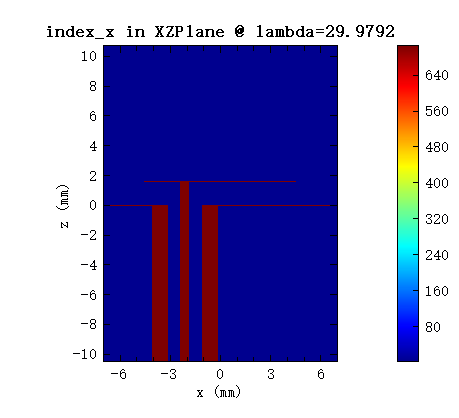
本案例中光源的波长范围为 相对于结构来说非常大,使用自动非均匀网格时,软件默认的网格精度为已无法满足仿真需求。因此我们在天线的矩形基板上增加了精细的网格覆盖,其余仿真区域的网格精度为4。下图为XZ平面Y=0处的Index监视器得到的 index_x 分布图,可以看到结构得到了正确的构建。
远场方向性分析组
方向性分析组用于设置监测器和计算贴片天线的方向性。由于这里使用的是无限接地平面,因此在分析组的 Setup Variables选项卡中的 inf_ground_plane 变量应该设置为 1。您可以点击远场分析:方向性来了解如何计算在无限接地平面上辐射的偶极子源的方向性。
仿真结果
反射
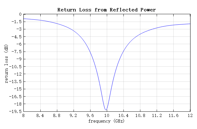
打开 rectangular_patch.mpps 文件并运行仿真后,rectangular_patch.msf 脚本将用于生成贴片天线的性能和辐射性能。从同轴波导中的port 1(S11)看到的反射(回波损耗=10log10|S11|)如下图。从中可以看到仿真出的贴片天线的谐振频率为 ,与理论谐振频率 相差 。
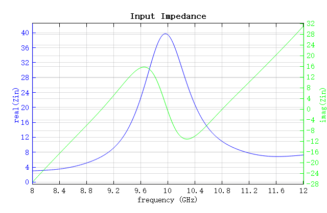
rectangular_patch.msf 脚本还可以得到天线的输入阻抗,如下图。可以看到天线的输入阻抗在谐振频率下达到 。
方向性
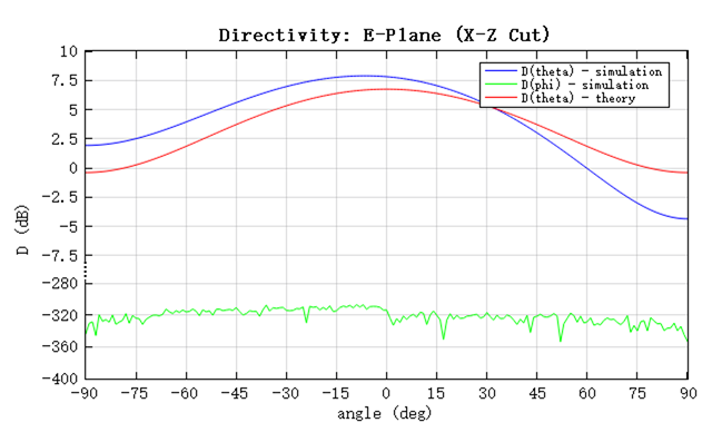
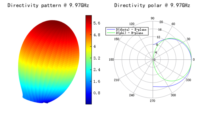
方向性分析组用于计算共振频率下的远场。rectangular_patch.msf 脚本会运行分析组并生成天线在E平面(XZ平面)和H平面(YZ平面)上的方向性分布图,并将其于理论[1:1]对比,如下图。在E平面上,理论和仿真出的 大致吻合, 远低于 ,与理论吻合。
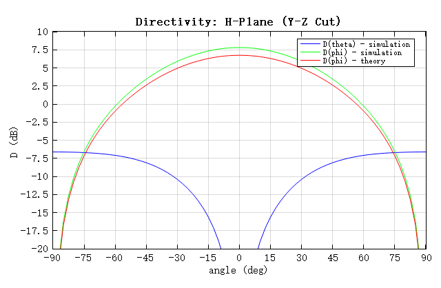
在 H 平面上,仿真结果和理论得到的 非常接近,如下图。
可以将E平面以及H平面的方向性画在极坐标的图中,如下图。E平面的不对称是由于馈电位置再ZX面的不对称导致的。
辐射性能
运行rectangular_patch.msf 脚本后天线的辐射性能将会自动显示在脚本行命令窗口中,结果如下:
============Radiation Performance==============
Resonant Frequency: 9.97 GHz
Input Power: 1.26 nW
Accepted Power: 1.24 nW
Radiated Power: 1.24 nW
Radiation Efficiency from Input Power: 98.8 Percent
Radiation Efficiency from Accepted Power: 100 Percent
Maximum Directivity: 7.88 dB
Total Realized Gain: 7.83 dB
=======================================
由于谐振频率下的 值非常小,因此输入功率和接收功率相等。因此,两种定义的辐射效率值大致相等。